Synthetic Difference-in-Differences as a Local Two-Way Fixed Effects Model

Oct 8, 2026 9 min read Causal Inference

Contents

Synthetic difference-in-differences (SDID; Arkhangelsky et al., 2021) is a two-way fixed effects (TWFE) regression fitted by weighted least squares. Each cell $(i, t)$ of the panel gets weight $\hat\omega_i \hat\lambda_t$, and the weights are chosen so that the fit concentrates on control units that track the treated units before treatment, and on pre-treatment periods that resemble the post-treatment periods. That is the sense in which SDID is a local TWFE model

In these notes, I first write DiD, synthetic control and SDID as one weighted regression, then look at where the weights come from. Two connections follow: SDID combines a TWFE outcome model with balancing weights, which gives it a doubly robust structure, and it is a local alternative to matrix completion. Finally, we check in R that SDID really is a weighted TWFE.

Setup and notation

Balanced panel: $N$ units, $T$ periods. The first $N_{co}$ units are controls and the last $N_{tr}$ are treated. Treatment starts after period $T_{pre}$, leaving $T_{post}$ post-treatment periods. Let $W_{it} = 1$ if unit $i$ is treated and $t > T_{pre}$, and $0$ otherwise.

Three estimators, one weighted regression

Recall weighted least squares: minimize $\sum_k w_k (y_k - x_k'b)^2$. Observations with larger $w_k$ pull the fit harder, and observations with $w_k = 0$ drop out entirely. The model stays the same; only the weights decide where it has to fit well.

DiD, synthetic control and SDID are all weighted least squares problems of the same form.

DiD / TWFE: unit and time fixed effects, equal weights:

$$ (\hat\tau^{did}, \hat\mu, \hat\alpha, \hat\beta) = \arg\min_{\tau,\mu,\alpha,\beta} \sum_{i=1}^{N}\sum_{t=1}^{T} \left(Y_{it} - \mu - \alpha_i - \beta_t - W_{it}\tau\right)^2 . $$

Synthetic control (SC): unit weights, but no unit fixed effect:

$$ (\hat\tau^{sc}, \hat\mu, \hat\beta) = \arg\min_{\tau,\mu,\beta} \sum_{i=1}^{N}\sum_{t=1}^{T} \left(Y_{it} - \mu - \beta_t - W_{it}\tau\right)^2 \hat\omega_i^{sc} . $$

SDID: TWFE model with unit weights and time weights:

$$ (\hat\tau^{sdid}, \hat\mu, \hat\alpha, \hat\beta) = \arg\min_{\tau,\mu,\alpha,\beta} \sum_{i=1}^{N}\sum_{t=1}^{T} \left(Y_{it} - \mu - \alpha_i - \beta_t - W_{it}\tau\right)^2 \hat\omega_i \hat\lambda_t . $$

Read the SDID line as the TWFE model, with observation weight $\hat\omega_i \hat\lambda_t$.

Side by side:

	Unit FE `$\alpha_i$`	Unit weights	Time weights
DiD	✓	`$1/N_{co}$`	`$1/T_{pre}$`
SC	✗	`$\hat\omega^{sc}$`	`$1/T_{pre}$`
SDID	✓	`$\hat\omega$`	`$\hat\lambda$`

The weights shown are for control units and pre-treatment periods. In all three, treated units get $1/N_{tr}$ and post-treatment periods get $1/T_{post}$.

Two observations:

SDID vs. DiD. With the weights, parallel trends only needs to hold for the comparison the weights pick out, not for every control unit and every pre-period.
SDID vs. SC. SDID does not need the convex hull. With $\alpha_i$ in the model, the synthetic control part in SDID only has to match the treated trajectory up to a constant shift, not its level. In contrast, SC must match levels exactly, which is why it struggles when the treated unit is outside the convex hull of controls.

Where the weights come from

Unit weights: a synthetic control with an intercept

$$ (\hat\omega_0, \hat\omega) = \arg\min_{\omega_0 \in \mathbb{R},\, \omega \in \Omega} \sum_{t=1}^{T_{pre}} \left( \omega_0 + \sum_{i=1}^{N_{co}} \omega_i Y_{it} - \frac{1}{N_{tr}} \sum_{i = N_{co}+1}^{N} Y_{it} \right)^2 + \zeta^2 T_{pre} \lVert \omega \rVert_2^2 , $$

where

$\Omega = \{\omega \in \mathbb{R}_+^{N_{co}} : \sum_i \omega_i = 1\}$.
$\zeta$ is a regularization parameter.
Treated units get $\hat\omega_i = 1/N_{tr}$.
The intercept $\omega_0$ is the unit fixed effect showing up in the weight problem: match the treated pre-trend up to a level shift.

Time weights: the same idea, turned sideways

$$ (\hat\lambda_0, \hat\lambda) = \arg\min_{\lambda_0 \in \mathbb{R},\, \lambda \in \Lambda} \sum_{i=1}^{N_{co}} \left( \lambda_0 + \sum_{t=1}^{T_{pre}} \lambda_t Y_{it} - \frac{1}{T_{post}} \sum_{t = T_{pre}+1}^{T} Y_{it} \right)^2 , $$

with $\Lambda$ the simplex over pre-periods. Post-treatment periods get $\hat\lambda_t = 1/T_{post}$.

This is a “synthetic pre-period”: the combination of pre-periods that best predicts, across control units, what the post-period looks like, again up to a constant $\lambda_0$, the echo of the time fixed effect. Pre-periods that look nothing like the post-period get little or no weight.

The closed form: a weighted 2×2 DiD

Because the weights are a product $\hat\omega_i \hat\lambda_t$ over a block design, the weighted TWFE coefficient collapses to a familiar 2×2 DiD, with weighted averages in each cell:

$$ \hat\tau^{sdid} = \underbrace{\left( \frac{1}{T_{post}}\sum_{t > T_{pre}} \bar Y_{tr,t} - \sum_{t \le T_{pre}} \hat\lambda_t \bar Y_{tr,t} \right)}_{\text{treated: post minus synthetic pre}} - \underbrace{\sum_{i=1}^{N_{co}} \hat\omega_i \left( \frac{1}{T_{post}}\sum_{t > T_{pre}} Y_{it} - \sum_{t \le T_{pre}} \hat\lambda_t Y_{it} \right)}_{\text{synthetic control: post minus synthetic pre}}, $$

where $\bar Y_{tr,t} = \frac{1}{N_{tr}} \sum_{i > N_{co}} Y_{it}$. Set $\hat\omega_i = 1/N_{co}$ and $\hat\lambda_t = 1/T_{pre}$, and you recover textbook DiD.

A doubly robust view

Combining outcome modeling with balancing weights, and the double robustness that comes with it, is one of the most prominent themes in the causal inference literature: AIPW in the cross-section (Robins, Rotnitzky & Zhao, 1994), doubly robust DiD (Sant’Anna & Zhao, 2020), and the augmented synthetic control method (Ben-Michael, Feller & Rothstein, 2021).

SDID fits this pattern. Its outcome model is TWFE, and its balancing weights are the unit and time weights. If either outcome modeling or weighting is correct, SDID is consistent.

The paper adds that the two sets of weights back each other up: even if one of them fails to remove the bias, the combination of unit and time weights can compensate. The authors themselves compare this to augmented inverse probability weighting, where one can trade off accuracy between the outcome model and the treatment assignment model. For the formal results, see Arkhangelsky et al. (2021).

SDID vs. matrix completion: local vs. global

Matrix completion (MC; Athey et al., 2021) starts from the same picture: the matrix of untreated outcomes $\mathbf{Y}(0)$ has its treated block missing, and it is approximately low rank. The two methods use that picture differently.

MC models the whole matrix. It estimates a low-rank $\mathbf{L}$ from all untreated cells and reads the treated block’s counterfactual off the fitted matrix. It tries to get things right everywhere: every unit, every period. The ATT is a by-product of the global fit.
SDID only needs one number: the average untreated outcome in the treated block. So it only needs things right locally: in the post-treatment periods, for units similar to the treated units. The weights select those units and periods, and the fixed effects absorb level differences.

A statistics analogy: estimating a whole regression function versus estimating its value at one point. For the single point, a fit that is accurate near that point is enough.

Neither dominates. MC returns a counterfactual for every cell, which is useful for unit-level effects and irregular treatment patterns. SDID targets the ATT directly and keeps a 2×2 interpretation. See also GSC through PCA for the hard-rank cousin of MC.

Seeing it in R: SDID really is weighted TWFE

We use the California Proposition 99 data shipped with synthdid (Abadie, Diamond & Hainmueller, 2010): cigarette packs per capita, 39 states, 1970–2000, California treated from 1989.

# remotes::install_github("synth-inference/synthdid")
library(synthdid)
library(tidyverse)
library(fixest)

Step 1: estimate SDID the standard way

data("california_prop99")

setup <- panel.matrices(california_prop99)   # Y matrix: controls first, treated last
tau_sdid <- synthdid_estimate(setup$Y, setup$N0, setup$T0)
tau_sdid

## synthdid: -15.604 +- NA. Effective N0/N0 = 16.4/38~0.4. Effective T0/T0 = 2.8/19~0.1. N1,T1 = 1,12.

Step 2: look at the learned weights

The estimator learns weights only for control units and pre-treatment periods, so those are the ones worth looking at.

w  <- attr(tau_sdid, "weights")
N0 <- setup$N0
T0 <- setup$T0

ctrl_w <- tibble(State = rownames(setup$Y)[1:N0], omega = w$omega)

pre_w  <- tibble(Year = as.integer(colnames(setup$Y)[1:T0]), lambda = w$lambda)

ctrl_w |> filter(omega > 0) |> arrange(desc(omega))

## # A tibble: 28 × 2
##    State          omega
##    <chr>          <dbl>
##  1 Nevada        0.124 
##  2 New Hampshire 0.105 
##  3 Connecticut   0.0783
##  4 Delaware      0.0704
##  5 Colorado      0.0575
##  6 Illinois      0.0534
##  7 Nebraska      0.0479
##  8 Montana       0.0451
##  9 Utah          0.0415
## 10 New Mexico    0.0406
## # ℹ 18 more rows

pre_w |> filter(lambda > 0)

## # A tibble: 3 × 2
##    Year lambda
##   <int>  <dbl>
## 1  1986  0.366
## 2  1987  0.206
## 3  1988  0.427

The two sets of weights are local in different degrees. In units, 28 of 38 control states get positive weight, and the top five carry 44% of it. In time, the weights are much more concentrated: only 3 of 19 pre-treatment years, all just before treatment, get positive weight.

Step 3: run a plain weighted TWFE

Treated units and post-treatment periods get uniform weights, $1/N_{tr}$ and $1/T_{post}$.

N1 <- nrow(setup$Y) - N0
T1 <- ncol(setup$Y) - T0

unit_w <- bind_rows(
  ctrl_w,
  tibble(State = rownames(setup$Y)[-(1:N0)], omega = 1 / N1)
)

time_w <- bind_rows(
  pre_w,
  tibble(Year = as.integer(colnames(setup$Y)[-(1:T0)]), lambda = 1 / T1)
)

panel_w <- california_prop99 |>
  left_join(unit_w, by = "State") |>
  left_join(time_w, by = "Year") |>
  mutate(wt = omega * lambda) |>
  filter(wt > 0)                          # zero-weight cells contribute nothing

twfe_local  <- feols(PacksPerCapita ~ treated | State + Year,
                     data = panel_w, weights = ~ wt)
twfe_global <- feols(PacksPerCapita ~ treated | State + Year,
                     data = california_prop99)

tibble(
  estimator = c("SDID (synthdid)", "Local TWFE (weighted feols)", "Global TWFE / DiD"),
  tau       = c(as.numeric(tau_sdid),
                coef(twfe_local)[["treated"]],
                coef(twfe_global)[["treated"]])
)

## # A tibble: 3 × 2
##   estimator                     tau
##   <chr>                       <dbl>
## 1 SDID (synthdid)             -15.6
## 2 Local TWFE (weighted feols) -15.6
## 3 Global TWFE / DiD           -27.3

The first two rows agree: SDID is the TWFE coefficient under weights $\hat\omega_i \hat\lambda_t$. The third row is what you get if you insist that parallel trends hold globally.

A caveat on inference: the standard errors feols reports for the weighted regression are not valid for SDID, because they treat the weights as fixed when they were estimated from the same data. Use vcov(tau_sdid, method = "placebo") with one treated unit, or the bootstrap or jackknife with several.

Step 4: look at the localization

synthdid_plot(tau_sdid)

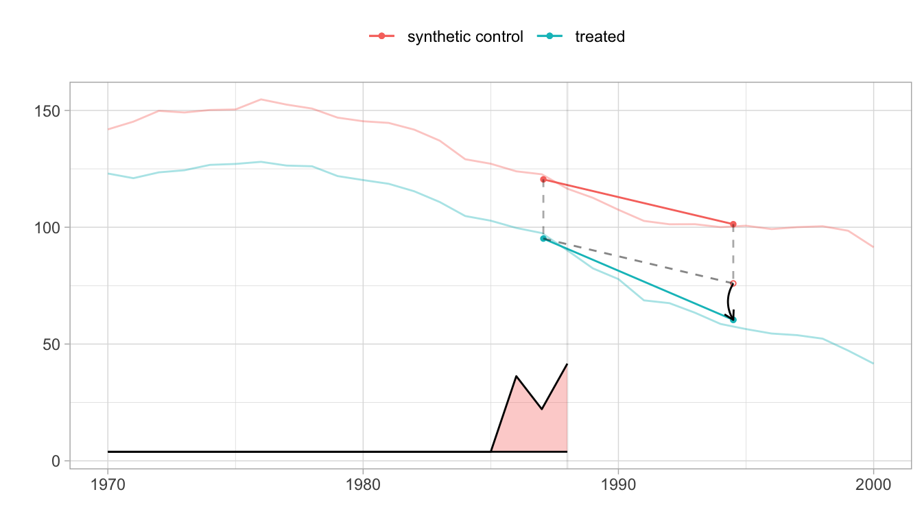
The shaded ribbon at the bottom of the plot is $\hat\lambda$: the pre-periods the estimator actually uses. The two lines are the treated unit and its synthetic control. They are parallel, not identical, in the weighted pre-period, which is exactly what the unit fixed effect allows.

References

Abadie, A., Diamond, A., & Hainmueller, J. (2010). Synthetic control methods for comparative case studies. Journal of the American Statistical Association, 105(490), 493–505.
Arkhangelsky, D., Athey, S., Hirshberg, D. A., Imbens, G. W., & Wager, S. (2021). Synthetic difference-in-differences. American Economic Review, 111(12), 4088–4118.
Athey, S., Bayati, M., Doudchenko, N., Imbens, G., & Khosravi, K. (2021). Matrix completion methods for causal panel data models. Journal of the American Statistical Association, 116(536), 1716–1730.
Ben-Michael, E., Feller, A., & Rothstein, J. (2021). The augmented synthetic control method. Journal of the American Statistical Association, 116(536), 1789–1803.
Robins, J. M., Rotnitzky, A., & Zhao, L. P. (1994). Estimation of regression coefficients when some regressors are not always observed. Journal of the American Statistical Association, 89(427), 846–866.
Sant’Anna, P. H. C., & Zhao, J. (2020). Doubly robust difference-in-differences estimators. Journal of Econometrics, 219(1), 101–122.

synthetic control difference-in-differences panel data doubly robust balancing weights

Chen Xing

Ph.D. Candidate in Marketing

Research: Sustainable luxury retailing · Causal inference · Causal machine learning

	Unit FE `\(\alpha_i\)`	Unit weights	Time weights
DiD	✓	`\(1/N_{co}\)`	`\(1/T_{pre}\)`
SC	✗	`\(\hat\omega^{sc}\)`	`\(1/T_{pre}\)`
SDID	✓	`\(\hat\omega\)`	`\(\hat\lambda\)`