Generalized Synthetic Control, Seen Through PCA
Contents
The generalized synthetic control (GSC) method of Xu (2017) is easy to understand as PCA1 with a missing block. These notes walk through each step and, for each one, say which part of the panel it uses. Covariates are assumed to be partialled out already, so the outcome is a pure factor structure.
1. Setup
Units $i \in \mathcal{C}$ (controls, $N_{co}$ of them) are never treated. Units $i \in \mathcal{T}$ (treated) are treated after period $T_0$. Untreated outcomes follow a factor model:
The target is the treated units’ untreated outcomes after $T_0$, giving
$$\widehat{ATT}_t = \frac{1}{|\mathcal{T}|} \sum_{i \in \mathcal{T}} \big( Y_{it} - \widehat{Y}_{it}(0) \big), \qquad t > T_0 .$$
Arrange the outcomes as a units-by-periods matrix. It has four blocks:
Pre: $t \le T_0$ |
Post: $t > T_0$ |
|
|---|---|---|
Controls $\mathcal{C}$ |
A observed | B observed |
Treated $\mathcal{T}$ |
C observed | D missing $Y_{it}(0)$, target |
GSC fills D in three steps: A + B, then C, then D.
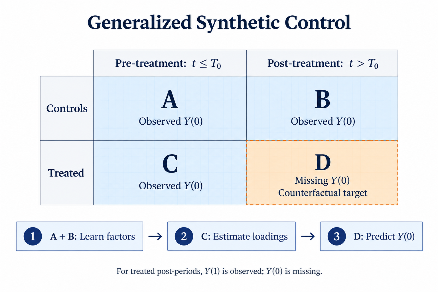
2. The PCA analogy
Put the control outcomes in a matrix $Y_{\mathcal{C}}$ with units in rows and periods in columns ($N_{co} \times T$). Each row is one unit’s whole trajectory. PCA is the eigen-decomposition of the $T \times T$ cross-product matrix $Y_{\mathcal{C}}' Y_{\mathcal{C}}$:
- Eigenvectors = factors. Each eigenvector has one entry per period, so it is a time path: a common trend shape shared across units. Stack the top
$r$eigenvectors as columns and you get$\widehat F$($T \times r$); row$t$of$\widehat F$is$\hat f_t'$. - Projections = loadings. A unit’s coordinates on these eigenvectors,
$\hat\lambda_i = \widehat F' Y_i$, say how much of each trend shape it carries. So$Y_{it} \approx \hat\lambda_i' \hat f_t$: every trajectory is a weighted sum of a few common time paths. - Eigenvalues = factor strength. The
$k$-th eigenvalue measures how much cross-unit variation the$k$-th time path explains. A few large eigenvalues mean a few strong factors.
Matching names in R. prcomp() stores the eigenvectors in $rotation and each unit’s projections on them in $x; PCA texts call $x the principal-component scores. Careful: many PCA texts call the eigenvectors “loadings”, while in GSC “loadings” means the unit-level projections.
| Object | prcomp(Y) output |
Dimension | GSC name |
|---|---|---|---|
eigenvectors of $Y'Y$ |
pca$rotation |
$T \times r$ |
factors $\widehat F$ |
| scores (projections on eigenvectors) | pca$x |
$N_{co} \times r$ |
loadings $\hat\lambda_i$ |
| eigenvalues | pca$sdev^2 |
one per component | factor strength |
For a treated unit, only the first $T_0$ coordinates of its trajectory are untreated. GSC computes its projection from those coordinates alone (Step 2), then rebuilds the missing coordinates from the eigenvectors (Step 3).
prcomp(..., center = TRUE) would additionally remove period means, which is the same as adding time fixed effects.
3. Step by step
Step 1: Learn the factors from controls (blocks A + B)

Run PCA on the control units over all periods and keep the first $r$ components:
$$\widehat{F} = (\hat f_1, \dots, \hat f_T)' \in \R^{T \times r} \quad \text{from} \quad Y_{\mathcal{C}} \approx \Lambda_{\mathcal{C}} F' , \ \operatorname{rank} = r .$$
pca   <- prcomp(Y, center = FALSE, rank. = r,
                data = {i: control units, t: all periods})
F_hat <- pca$rotation   # eigenvectors, T x r -> GSC factors
Treated units play no role here, so treatment cannot contaminate $\widehat{F}$. The block is complete, so a single SVD suffices; no iteration is needed.
Step 2: Fit each treated unit’s loadings (block C)
For each treated unit, regress its pre-treatment outcomes on the estimated factors, period by period:
$$\hat\lambda_i = \big( \widehat{F}_{\text{pre}}' \widehat{F}_{\text{pre}} \big)^{-1} \widehat{F}_{\text{pre}}' \, Y_{i,\text{pre}}, \qquad i \in \mathcal{T}.$$
lm(Y_it ~ f1_t + ... + fr_t - 1,
   data = {i: treated unit i, t: pre-treatment periods})
In PCA terms this is predict(pca, newdata), except the new unit has only $T_0$ of its $T$ coordinates observed. The projection becomes a regression on the matching rows of $\widehat{F}$, and $T_0$ needs to be comfortably larger than $r$.
Step 3: Reconstruct the missing block (block D)
Combine the treated loadings with the post-period factors:
$$\widehat{Y}_{it}(0) = \hat\lambda_i' \hat f_t, \qquad i \in \mathcal{T}, \ t > T_0 .$$
Y0_hat <- predict(fit_i,
  newdata = {i: treated unit i, t: post-treatment periods})
$\widehat{ATT}_t$ follows from the formula in Section 1.
Choosing the number of factors (block C again)
The only tuning parameter is the number of factors $r$, and it is chosen before Steps 2–3. For each candidate $r$:
- Keep
$\widehat{F}$from Step 1. - Hold out one pre-period
$s \le T_0$for all treated units. - Refit Step 2 on the remaining pre-periods.
- Predict
$Y_{is}$and record the error. - Loop over all
$s$to get the MSPE.
Pick the $r$ with the smallest MSPE.
lm(Y_it ~ f1_t + ... + fr_t - 1,
   data = {i: treated unit i, t: pre-treatment periods, t != s})
# error at {i: treated unit i, t: s}
The validation cells are untreated outcomes of the treated units. They mimic the prediction problem in block D more closely than control cells would.
Summary of data use
| Step | Task | Units | Periods | Block |
|---|---|---|---|---|
| 1 | factors $\widehat F$ |
controls | all | A + B |
| 2 | loadings $\hat\lambda_i$ |
treated | pre | C |
| 3 | impute $\widehat Y_{it}(0)$ |
treated | post | D |
| CV | choose $r$ |
treated | pre, leave one out | C |
In R, the whole pipeline is
library(gsynth)
gsynth(Y ~ D, data = df, index = c("id", "time"),
       force = "none", CV = TRUE, r = c(0, 5))
4. Relation to matrix completion
Both methods treat $Y(0)$ as a low-rank matrix $L$ plus noise and impute the missing cells. Write $\mathcal{O}$ for all observed untreated cells (A + B + C). They differ in how rank is controlled, which is easiest to see through the singular values $\sigma_1 \ge \sigma_2 \ge \dots$ of $L$. These are the square roots of the eigenvalues in Section 2, so they also measure factor strength.
Statistics analogy: the rank $\operatorname{rank}(L) = \|\sigma\|_0$ is an $L_0$ norm on the singular values, and the nuclear norm $\|L\|_* = \|\sigma\|_1$ is an $L_1$ norm. GSC versus matrix completion is best subset versus lasso, applied to singular values instead of coefficients.
GSC / IFE (hard-impute). Constrain the rank explicitly to $r$:
$$\min_{L} \sum_{(i,t) \in \mathcal{O}} (Y_{it} - L_{it})^2 \quad \text{s.t.} \quad \operatorname{rank}(L) \le r .$$
The SVD keeps the top $r$ singular values unchanged and sets the rest to zero:
$$\mathcal{H}_r(\sigma_k) = \sigma_k \, \1\{k \le r\}.$$
The problem is non-convex. $r$ is chosen by cross-validation, and the implicit belief is that a few strong, discrete factors drive the data. GSC approximates this problem in two blocks rather than solving it jointly: A + B pins down $F$, and C only pins down $\lambda_i$. Fitting all of $\mathcal{O}$ jointly by iterating hard-thresholded SVDs is the EM variant (EM = TRUE in gsynth).
Matrix completion (soft-impute; Athey et al. 2021). Replace the rank constraint with its tightest convex relaxation, the nuclear norm:
$$\min_{L} \sum_{(i,t) \in \mathcal{O}} (Y_{it} - L_{it})^2 + \lambda \|L\|_*, \qquad \|L\|_* = \sum_k \sigma_k .$$
Each iteration shrinks every singular value toward zero by the same amount:
$$\mathcal{S}_\lambda(\sigma_k) = \max(0, \sigma_k - \lambda).$$
Small components are zeroed and large ones are kept but attenuated. There is no hard cutoff, so weaker factors can still contribute. $\lambda$ is chosen by cross-validation on held-out observed cells.
| GSC (Xu 2017) | Matrix completion (Athey et al. 2021) | |
|---|---|---|
| Rank control | hard: $\operatorname{rank}(L) \le r$ |
soft: nuclear-norm penalty |
| Singular values | keep top $r$, drop the rest |
shrink all by $\lambda$ |
Cells used to learn $F$ |
controls only (A + B) | all observed untreated cells (A + B + C) |
| Treatment pattern | block: common or staggered start, never-treated controls | any missing pattern |
| Tuning | $r$, CV on treated pre-periods |
$\lambda$, CV on observed cells |
In gsynth |
estimator = "ife" |
estimator = "mc" |
The summary: GSC is matrix completion with a hard rank constraint, fitted in two blocks. Swap the rank constraint for the nuclear norm, and let block C inform the factors as well, and you arrive at matrix completion.
5. When to use which
Start with the eigenvalues of the control block: plot(pca) gives the scree plot.
- Few strong factors: GSC. A few large eigenvalues followed by a clear gap. Outcomes are driven by a small number of distinct common shocks, such as a major federal policy change or a few distinct regional economic cycles. Truncation isolates that factor subspace and leaves the retained singular values unshrunk, so the signal is not biased toward zero. Soft-impute would shrink these large singular values by
$\lambda$as well. - Many weak factors: matrix completion. Eigenvalues decay slowly with no clear gap. Confounding comes from many small, diffuse trends, such as multi-sector economic drift or micro-level behavioral patterns. Any hard cutoff
$r$either drops real signal or fits noise. Continuous shrinkage keeps weak components at reduced weight, which typically gives better recovery of$L$and lower MSE. - Shape of the data. GSC needs never-treated controls and enough pre-periods per treated unit (
$T_0$well above$r$). With few controls, short pre-periods or an irregular treatment pattern, matrix completion gains from also learning the factors from block C.
In the lasso analogy: best subset wins when a few coefficients are large and the rest are exactly zero, and the lasso wins when many coefficients are small but nonzero. When the scree plot is ambiguous, fit both and compare their cross-validated prediction error on held-out untreated cells.
References
- Xu, Y. (2017). Generalized synthetic control method: Causal inference with interactive fixed effects models. Political Analysis, 25(1), 57–76.
- Bai, J. (2009). Panel data models with interactive fixed effects. Econometrica, 77(4), 1229–1279.
- Athey, S., Bayati, M., Doudchenko, N., Imbens, G., & Khosravi, K. (2021). Matrix completion methods for causal panel data models. Journal of the American Statistical Association, 116(536), 1716–1730.
- Mazumder, R., Hastie, T., & Tibshirani, R. (2010). Spectral regularization algorithms for learning large incomplete matrices. Journal of Machine Learning Research, 11, 2287–2322.
Related notes: Interactive Fixed Effects, Matrix Completion, Synthetic Control.
-
The intuition behind PCA is dimension reduction: PCA reduces dimension by projecting a high-dimensional point cloud onto a few directions. A good projection keeps the points “spread out” instead of collapsing them together, and variance measures that spread. The directions with the most spread are the eigenvectors of the data’s covariance matrix. Each eigenvalue tells you how much variance its direction captures, so keeping the eigenvectors with the largest eigenvalues keeps the most important structure. ↩︎

Chen Xing
Ph.D. Candidate in Marketing
Research: Sustainable luxury retailing · Causal inference · Causal machine learning