Notes on Callaway & Sant’Anna (2021) – Staggered Adoption DiD
0. Motivation
Staggered‐adoption policies break the canonical two-period / two-group DiD model. It has been shown that the traditional two-way fixed-effects (TWFE) regression can assign negative weights to treatment effects, thereby obscuring their dynamic and heterogeneous patterns.
Callaway & Sant’Anna (2021) propose a divide-and-conquer strategy:
-
Divide the messy staggered panel into many honest $2\times2$ DiDs
-
Conquer by estimating each “little” DiD under familiar assumptions, then combine them with user-chosen weights to answer specific questions
The key takeaway:
-
Use $\operatorname{ATT}(g, t)$ as a building block so we can transparently see how things are constructed
-
Many different aggregation schemes are possible: they deliver different parameters
-
Can allow for covariates via regressions adjustments, IPW, and DR.
1. Setup
-
Data structure: Panel of units $i$ over time $t = 1,\dots,T$
-
Let $D_{it}$ be a binary variable. $D_{it} = 1$ if unit $i$ is treated in period $t$; $D_{it} = 0$ otherwise
-
Cohorts
-
Define $G$ as the time period when a unit first becomes treated. For all units that eventually get treated, $G$ defines which “group” they belong to
-
Define $G_{g}$ as a binary variable. $G_{g} = 1$ if a unit is first treated in period $g$ (i.e. $G_{i,g} = \1\{G_i = g\}$ )
-
Define $G=\infty$ as “never treated” group.
-
-
Potential outcomes
-
$Y_{it}(g)$: outcome at time $t$ if first treated in period $g$.
-
$Y_{it}(\infty)$: outcome if never treated.
-
-
Cohort-time ATT
Assume $\mathrm{iid}$, drop unit index $i$. A parameter of interest that has clear interpretation is the $\operatorname{ATT}(g, t)$: $$ \operatorname{ATT}(g, t)=\mathbb{E}\left[Y_t(g)-Y_t(\infty) \mid G_g=1\right], \text { for } t \geq g . $$ This defines one “clean” $2\times2$ DiD for each pair $(g,t)$.
Remark 1.Why focus on time after treatment starting period, $t \ge g$? Because we need the no anticipation assumption. Before treatment taking place, $t < g$, there is no treatment effect.
2. Key Assumptions
Given that we never observe $Y(\infty)$ in post-treatment periods among units that have been treated, we need to make assumptions to identify $\operatorname{ATT}(g, t)$.
The no anticipation assumption has exactly the same content as in the $2\times2$ case.
Note that, (1) is equivalent to the following: for $t \in\{2, \ldots, T\}, g \in \mathcal{G}, t \geq g$ ,
$$ \mathbb{E}\left[Y_t(\infty)-Y_{g-1}(\infty) \mid G_g=1\right]=\mathbb{E}\left[Y_t(\infty)-Y_{g-1}(\infty) \mid G=\infty\right], \tag{1’} $$
Similarly, (2) is equivalent to (2’), that is, changing $Y_{t-1}(\infty)$ to $Y_{g-1(\infty)}$ in (2).
3. Identification: Long-Difference Estimands
Under no anticipation and one of the parallel-trends assumptions, each $\mathrm{ATT}(g,t)$ equals a simple long-difference DID:
- Using never-treated
- Using not-yet-treated
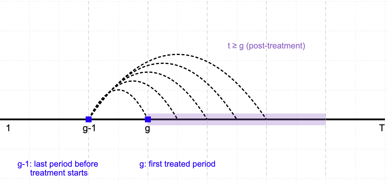
A: Longer Time Span! Check my plot above. The "long difference" refers to the fact that the comparison often spans from a pre-treatment period (i.e. $g-1$) to a later period (post-treatment, $t \ge g$), potentially covering multiple time periods. This contrasts with "short differences," which might involve comparing outcomes in consecutive periods or shorter time windows.
For each treated cohort, the method computes the difference in outcomes between the pre-treatment period and a specific post-treatment period, potentially far apart in time. This extended gap emphasizes the "long" aspect, as it captures the cumulative effect of the treatment over time.
Moreover, with covariates, one can form doubly-robust estimators that combine generalized propensity scores $p_g(X_i)$ and outcome models $m_{g,t}(X_i)$. At high level, the form of this estimator is identical to AIPW–ATT in cross–section, but we need to replace “levels” (e.g. $Y$) with “changes” (e.g. $\Delta Y$).
For more details, check Theorem 1 in the paper.
4. Aggregation of $\mathrm{ATT}(g,t)$
Any overall summary $\theta$ is a weighted average of the cell-specific ATTs:
$$ \theta=\sum_{g=2}^T \sum_{t=g}^T w_{g, t} \operatorname{ATT}(g, t), \quad \sum_{g, t} w_{g, t}=1 . $$
Common choices:
- Cohort-heterogeneity: Average effect of participating in the treatment that units in group $g$ experienced,
-
Calendar time heterogeneity
-
Event-study / dynamic treatment effects
5. Limitation & Extension
Lee & Wooldridge (2023) argue that Callaway & Sant’Anna (2021) method is less efficient but more resilient to functional form of covariates. The followings are from their working paper:
… CS (2021) method uses only the period just prior to the intervention in defining the control group, thereby discarding potentially useful information in earlier time periods.
In fact, Wooldridge (2021) shows that, under the standard “error components” structure on the error, with a homoskedastic time-constant component and homoskedastic and serially uncorrelated idiosyncratic errors, the POLS estimator is both best linear unbiased (BLUE) and asymptotically efficient. These theoretical results imply that the CS (2021) estimators are inefficient under a standard set of assumptions. The simulations in Wooldridge (2021) bear this out, showing the CS approach can be very inefficient. Balanced against the loss in precision is that the CS approach can be less biased when parallel trends are violated.
To improve the efficiency, instead of using long differences, Lee and Wooldridge (2023) use all suitable control observations in transforming the outcome variable. Specifically, rather than using the single period just prior to the treatment, $Y_{g-1}$, they use the pre-treatment average, $\frac{1}{g-1}\sum_{s = 1}^{g-1}Y_s$.
The rolling method (Lee and Wooldridge, 2023) transforms panel data with staggered interventions by subtracting each unit’s average outcome across all pre-treatment periods from their outcome in the current period of interest. This transformation, combined with no anticipation and parallel trends assumptions, makes the treatment assignment unconfounded for the transformed outcome in each cohort/time cross-section. With unconfoundedness holding, we can then apply standard treatment effects estimators, including doubly robust methods and matching, utilizing all not-yet-treated units as the valid control group for that specific cross-section.
6. R code Example
The following R code example is provided by Professor Scott Cunningham.
library(readstata13)
library(ggplot2)
library(did) # Callaway & Sant'Anna

castle <- data.frame(read.dta13('https://github.com/scunning1975/mixtape/raw/master/castle.dta'))
castle$effyear[is.na(castle$effyear)] <- 0 # untreated units have effective year of 0

# Estimating the effect on log(homicide)
atts <- att_gt(yname = "l_homicide", # LHS variable
               tname = "year", # time variable
               idname = "sid", # id variable
               gname = "effyear", # first treatment period variable
               data = castle, # data
               xformla = NULL, # no covariates
               #xformla = ~ l_police, # with covariates
               est_method = "dr", # "dr" is doubly robust. "ipw" is inverse probability weighting. "reg" is regression
               control_group = "nevertreated", # set the comparison group which is either "nevertreated" or "notyettreated"
               bstrap = TRUE, # if TRUE compute bootstrapped SE
               biters = 1000, # number of bootstrap iterations
               print_details = FALSE, # if TRUE, print detailed results
               clustervars = "sid", # cluster level
               panel = TRUE) # whether the data is panel or repeated cross-sectional

# Aggregate ATT
agg_effects <- aggte(atts, type = "group")
summary(agg_effects)

# Group-time ATTs
summary(atts)

# Plot group-time ATTs
ggdid(atts)

# Event-study
agg_effects_es <- aggte(atts, type = "dynamic")
summary(agg_effects_es)

# Plot event-study coefficients
ggdid(agg_effects_es)
Reference
Callaway, Brantly and Pedro H. C. Sant’Anna (2021), “Difference-in-Differences with multiple time periods,” Journal of Econometrics, Themed Issue: Treatment Effect 1, 225 (2), 200–230.
Lee, S. J., & Wooldridge, J. M. (2023). A Simple Transformation Approach to Difference-in-Differences Estimation for Panel Data (SSRN Scholarly Paper No. 4516518). Social Science Research Network. https://doi.org/10.2139/ssrn.4516518
Sant’Anna, Pedro H. C. and Jun Zhao (2020), “Doubly robust difference-in-differences estimators,” Journal of Econometrics, 219 (1), 101–22.
How does doubly robust DiD estimator works? Check this: Lecture 5: How Covariates can make your DiD More Plausible
did R package 📦