AIPW vs. Residual-on-Residual regression: Non-Parametric Flexibility or Efficiency?

Jun 11, 2025 3 min read causal inference, econometrics

Introduction

Two powerful tools in causal inference are the Augmented Inverse Propensity Weighting (AIPW) estimator and the Residual-on-Residual regression estimator for partially linear models. Drawing from Wager’s notes (2024), this post breaks down how these estimators work, compares their strengths and weaknesses, and offers tips for when to use each.

Residual-on-Residual regression

The semiparamteric partially linear model (PLM) assumes the outcome $Y$ can be written as:

$\begin{matrix} (1) & Y = θ D + g (X) + ϵ \end{matrix}$

Here, $D$ is a binary treatment, $θ$ is the causal parameter of interest, $g (X)$ is some unknown function of covariates $X$ , and $ϵ$ is random noise with $E [ϵ ∣ D, X] = 0$ . The residual-on-residual estimator (or Robinson (1988) estimator) isolates $θ$ in two steps:

Partialing out covariates: “Partialing out” $X$ from $D$ and $Y$ using nonparametric regression and cross-fitting: $\tilde{D} = D - \hat{E} [D ∣ X]$ and $\tilde{Y} = Y - \hat{E} [Y ∣ X]$ .
Estimate the effect: Use linear regression $\tilde{Y} \sim \tilde{D}$ to get $\hat{θ}$ .

However, the model is not fully general, because it imposes a parametric specification on the key component of interest. It imposes additivity in

g (X)

and

D

Augmented Inverse Propensity Weighting (AIPW) Estimator

AIPW takes a fully non-parametric approach, aiming to estimate ATE, $τ = E [Y (1) - Y (0)]$ , where $Y (1)$ and $Y (0)$ are potential outcomes under treatment and control.

{\hat{τ}}_{AIPW} = \frac{1}{n} \sum_{i = 1}^{n} [{\hat{μ}}_{1} (X_{i}) - {\hat{μ}}_{0} (X_{i}) + D_{i} \frac{Y_{i} - {\hat{μ}}_{1} (X_{i})}{\hat{e} (X_{i})} - (1 - D_{i}) \frac{Y_{i} - {\hat{μ}}_{0} (X_{i})}{1 - \hat{e} (X_{i})}]

Here, ${\hat{μ}}_{1} (X)$ and ${\hat{μ}}_{0} (X)$ are outcome regression estimators for treated and untreated units, and $\hat{e} (X)$ is the estimator of propensity score. AIPW combines outcome modeling with inverse propensity weighting, making it doubly robust: it’s consistent if either the outcome model or propensity score is consistent.

The Key Difference: Non-Parametric vs. Partially Linear

AIPW is fully non-parametric, imposing no specific parametric form on the treatment effect, while residual-on-residual regression estimator assumes a partially linear structure

AIPW’s flexibility:
- AIPW does not assume a specific parametric form!
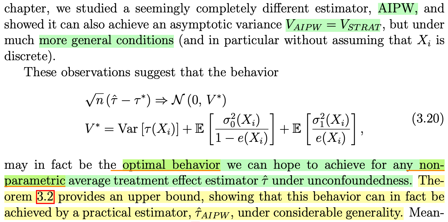
- AIPW is efficient in the generic non-parametric setting.
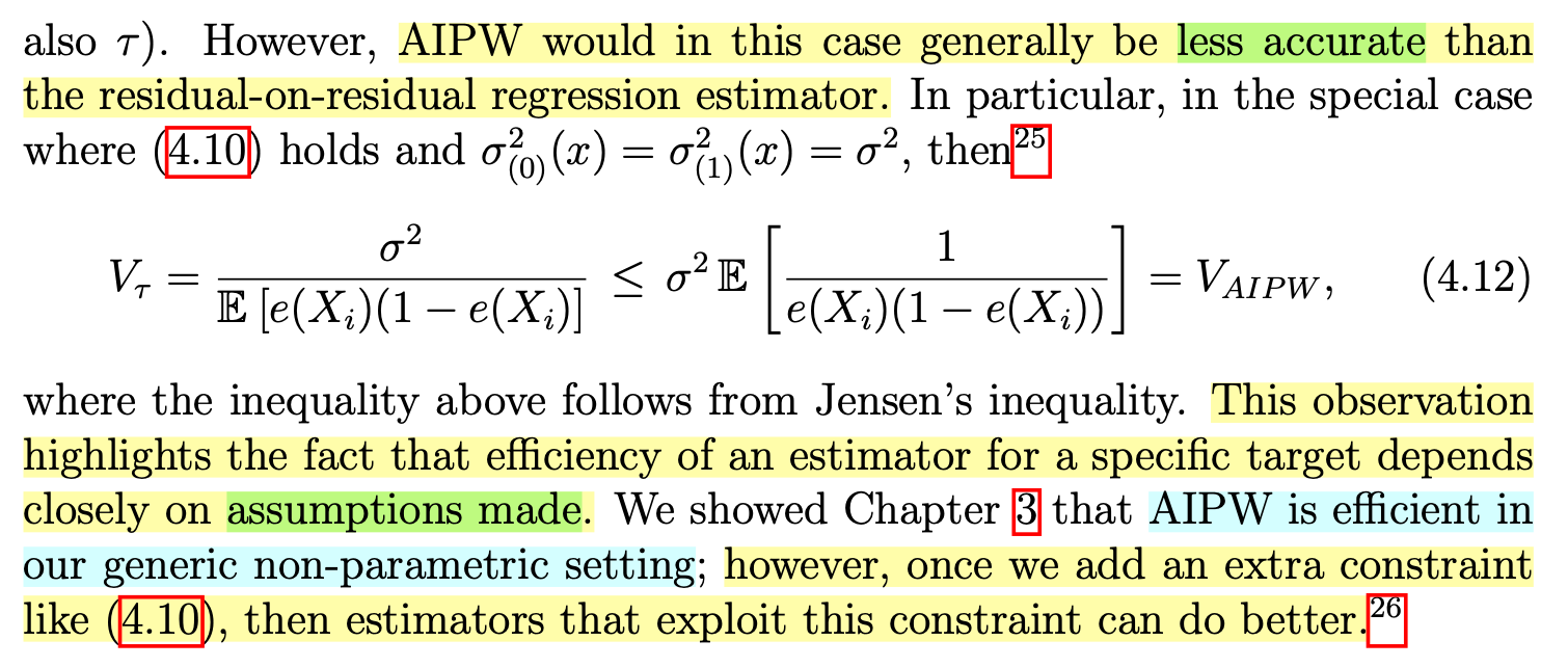
Residual-on-residual regression’s structure: What partially linear assumption buys us is that residual-on-residual estimators that exploit this constraint can have smaller variance than AIPW. In other words, adding this additional structure makes the residual-on-residual estimator more efficient than AIPW.

A risk of using the residual-on-residual estimator is that constant treatment effect model (1) may be misspecified.

Why This Matters

The choice between AIPW and residual-on-residual regression reflects a deeper trade-off in causal inference: flexibility versus efficiency. AIPW’s non-parametric nature makes it a Swiss Army knife for complex data, while PLM structure is like a precision tool—effective when conditions are right.

As Wager’s notes highlight:

Both AIPW and residual-on-residual regression are Neyman-orthogonal, making them robust to first‐stage errors.
However, their assumptions shape their performance. AIPW attains the lowest possible asymptotic variance for ATE under unconfoundedness. The residual-on-residual estimator, by imposing extra structure, can go beyond that bound when its structure is correct but at the cost of vulnerability to misspecification.

Conclusion

AIPW’s fully non-parametric approach offers robustness and flexibility, while residual-on-residual regression’s partially linear structure prioritizes efficiency when assumptions hold.

Reference

Wager, S. (2024). Causal inference: A statistical learning approach. https://web.stanford.edu/~swager/causal_inf_book.pdf

causal inference causal machine learning AIPW semiparametric partially linear model residual-on-residual cross-fitting Neyman orthogonality double robust double machine learning

Chen Xing

Founder & Data Scientist

Enjoy Life & Enjoy Work!