A walkthrough of how Causal Forest 🌲 works

Introduction

In this post, I will go over how causal forest works based on the tutorial in grf R package. Causal Forests offer a flexible, data-driven approach to estimating varied treatment effects, bridging machine learning and causal inference techniques.

Common Setting

If we are working on an observational study, we have the following data:

• Outcome variable: $Y_i$

• Binary treatment indicator: $W_i = \{0, 1\}$

• A set of covariates: $X_i$

Let’s assume that the following conditions hold:

1. (Assumption 1) $W_i$ is unconfounded given $X_i$ (i.e. treatment is as good as random given covariates).

$$\{Y_i(0), Y_i(1)\} \perp W_i | X_i$$

2. (Assumption 2) The confounders $X_i$ have a linear effect on $Y_i$.
3. (Assumption 3) The treatment effect $\tau$ is constant.

Then we could run a regression of the type

$$ Y_i = \tau W_i + \beta X_i + \epsilon_i $$

and interpret the estimate of $\hat{\tau}$ as the average treatment effect (ATE) $\tau = \mathbb{E}(Y_i(1) - Y_i(0))$.

Relaxing Assumptions

• Assumption 1 is an “identifying” assumption we have to live with

• Assumption 2 and Assumption 3 are modeling assumptions that we can question.

Relaxing Assumption 2: Partially Linear Model (PLR)

Assumption 2 is a strong parametric modeling assumption that requires the confounders to have a linear effect on the outcome, and that we should be able to relax by relying on semi-parametric statistics.

We can instead posit the partially linear model:

$$ Y_i = \tau W_i + f(X_i) + \epsilon_i, \ \ \ \mathbb{E}(\epsilon_i | X_i, W_i) = 0 $$

How do we get around estimating $\tau$ when we do not know $f(X_i)$?

Define the propensity score as $$e(x) = \mathbb{E}(W_i | X_i = x),$$

and the conditional mean of $Y$ as

$$m(x) = \mathbb{E}(Y_i | X_i = x) = f(x) + \tau e(x).$$

By Robinson (1988), we can rewrite the above equation in “centered” form:

$$Y_i - m(x) = \tau \cdot [W_i - e(x)] + \epsilon_i$$

This formulation has great practical appeal, as it means $\tau$ can be estimated by residual-on-residual regression.

Good properties 😀: Robinson (1988) shows that this approach yields root-n consistent estimates of $\tau$, even if estimates of $m(x)$ and $e(x)$ converge at a slower rate (“4-th root” in particular). This property is often referred to as orthogonality and is a desirable property that essentially tells you that given noisy “nuisance” estimates ($m(x)$ and $e(x)$) you can still recover “good estimates of your target parameter ($\tau$). For more details, please refer to Wager, Stefan “STATS 361: Causal Inference” Lecture 3.

But how to estimate $m(x)$ and $e(x)$?

• Use modern machine learning models! One could use boosting, random forest, and etc to estimate $m(x)$ and $e(x)$ because what we need is just “reasonable accurate” predictions, i.e.

$$\mathbb{E}\left[(\hat{m}(X)-m(X))^2\right]^{\frac{1}{2}}, \mathbb{E}\left[(\hat{e}(X)-e(X))^2\right]^{\frac{1}{2}}=o_P\left(\frac{1}{n^{1 / 4}}\right)$$

• Issue with Direct Plug-in of Estimates: Directly plugging in $\hat{m}(x)$ and $\hat{e}(x)$ into the residual-on-residual regression typically leads to bias because modern ML methods regularize to trade off bias and variance.

• Solution via Cross-Fitting: cross-fitting, where the prediction for observation $i$ is obtained without using unit $i$ for estimation, can help overcome this bias (Chernozhukov et al. 2018).

Relaxing Assumption 3: Non-constant treatment effects

Non-constant treatment effects occur when the impact of a treatment varies across different subgroups or individuals. This concept relaxes the assumption of homogeneous treatment effects, where the treatment is assumed to have the same impact on all units.

We could specify certain subgroups and run separate regressions for each subgroup and obtain different estimates of $\tau$. To avoid false discoveries, this approach would require us to specify potential subgroups without looking at the data. How can we use the data to inform us of potential subgroups?

Let’s define,

$$ Y_i=\textcolor{red}{ \tau\left(X_i\right) } D_i+f\left(X_i\right)+\varepsilon_i, \quad E\left[\varepsilon_i \mid X_i, D_i\right]=0, $$

where $\textcolor{red}{ \tau\left(X_i\right) }$ is the conditional ATE, i.e., $\textcolor{red}{ \tau\left(X_i\right) } :=\mathbb{E}\left[Y_i(1)-Y_i(0) \mid X_i\right]$. How do we estimate this?

Idea: If we imagine we had access to some neighborhood $\mathcal{N}(x)$ where $\tau$ was constant, we could proceed exactly as before, by doing a residual-on-residual regression on the samples belonging to $\mathcal{N}(x)$, i.e.:

$$ \tau(x) := \operatorname{lm}\left(Y_i - \hat{m}^{(-i)}(X_i) \sim W_i - \hat{e}^{(-i)}(X_i), \text{ weights } = 1\{X_i \in \mathcal{N}(x)\} \right) $$

This is conceptually what Causal Forest does, it estimates the treatment effect $\tau(x)$ for a target sample $X_i = x$ by running a weighted residual-on-residual regression on samples that have similar treatment effects.

These weights play a crucial role, so how does grf 📦 find them?

Random forest as an adaptive neighborhood finder

Breiman’s random forest for predicting the conditional mean $\mu(x) = \mathbb{E}(Y_i | X_i = x)$ can be briefly summarized in two steps:

1. Building phase: Build $B$ trees which greedily place covariate splits that maximize the squared difference in subgroups means

$$ n_L \cdot n_R \cdot ( \bar{y}_L - \bar{y}_R )^{2} $$

2. Prediction phase: Aggregate each tree’s prediction to form the final point estimate by averaging the outcomes $Y_i$ that fall into the same terminal leaf $L_b(X_i)$ as the targets sample $x$: $$\begin{align} \hat{\mu}(x) &= \sum_{i=1}^n \frac{1}{B} \sum_{b=1}^B Y_i \frac{1\left\{X i \in L_b(x)\right\}}{\left|L_b(x)\right|} \tag{1} \\ & =\sum_{i=1}^n Y_i \textcolor{blue}{\alpha_i(x)} \tag{2}, \end{align}$$ 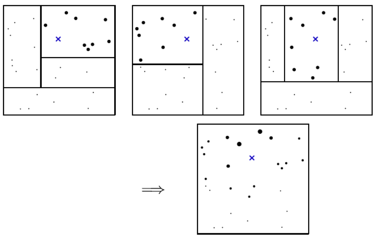Note that, this procedure is a double summation, first over trees, then over training samples (see equation (1)). We can swap the order of summation and obtain $\textcolor{blue}{\alpha_i(x)}$ in the equation (2). We have defined $\textcolor{blue}{\alpha_i(x)}$ as the frequency with which the $i$-th training sample falls into the same leaf as $x$.

The following image illustrates how the $\textcolor{blue}{\alpha_i(x)}$ are calculated: Some dots are larger because they are used by all trees, while some are smaller because they are only used by a few trees.

Causal Forest

Causal Forest essentially combines Breiman (2001) and Robinson (1988) by modifying the steps above to:

1. Building phase: Greedily places covariate splits that maximize the squared difference in subgroup treatment effects $$n_L \cdot n_R \cdot ( \hat{\tau}_L - \hat{\tau}_R )^{2},$$ where $\hat{\tau}$ is obtained by running Robinson’s residual-on-residual regression for each possible split point.

2. Use the resulting forest weights $\textcolor{blue}{\alpha_i(x)}$ to estimate $$\tau(x):=\operatorname{lm}\left(Y_i-\hat{\mu}^{(-i)}\left(X_i\right) \sim W_i-\hat{e}^{(-i)}\left(X_i\right), \text { weights }=\textcolor{blue}{\alpha_i(x)}\right),$$ where $\textcolor{blue}{\alpha_i(x)}$ capture how “similar” a target sample $x$ is to each of the training samples $X_i$

That is, Causal Forest is running a “forest”-localized version of Robinson’s regression. This adaptive weighting (instead of leaf-averaging) coupled with some other forest construction details known as “honesty” and “subsampling” can be used to give asymptotic guarantees for estimation and inference with random forests (Wager & Athey, 2018)

Efficiently estimating summaries of the CATEs

What about estimating summaries of $\tau(x)$, in terms of estimands like the average treatment effect (ATE), or the best linear projection (BLP), that have guaranteed $\sqrt{n}$ rate of convergence along with exact confidence intervals?

For estimating ATE, there are more efficient methods than simply averaging individual CATE estimates. Robins, Rotnitzky & Zhao (1994) showed that the so-called Augmented Inverse Probability Weighted (AIPW) estimator is asymptotically optimal for $\tau$ (meaning that among all non-parametric estimators, it has the lowest variance).

$$\begin{gathered} \hat{\tau}_{AIPW}=\frac{1}{n} \sum_{i=1}^n\left(\hat{\mu}_{(1)}\left(X_i\right)-\hat{\mu}_{(0)}\left(X_i\right)+\frac{W_i}{\hat{e}\left(X_i\right)}\left(Y_i-\hat{\mu}_{(1)}\left(X_i\right)\right)\right. \\ \left.-\frac{1-W_i}{1-\hat{e}\left(X_i\right)}\left(Y_i-\hat{\mu}_{(0)}\left(X_i\right)\right)\right), \end{gathered}$$

where $$\mu_{(w)}(x)=\mathbb{E}\left[Y_i \mid X_i=x, W_i=w\right]$$ and $$e(x)=\mathbb{P}\left[W_i=1 \mid X_i=x\right]$$

To interpret the AIPW estimator $\hat{\tau}_{AIPW}$ , it is helpful to decompose it into two components: Let $\hat{\tau}_{AIPW} = A + B$ , where

$$ A=\frac{1}{n} \sum_{i=1}^n\left(\hat{\mu}_{(1)}\left(X_i\right)-\hat{\mu}_{(0)}\left(X_i\right)\right) $$ $$ B=\frac{1}{n} \sum_{i=1}^n\left(\frac{W_i}{\hat{e}\left(X_i\right)}\left(Y_i-\hat{\mu}_{(1)}\left(X_i\right)\right)-\frac{1-W_i}{1-\hat{e}\left(X_i\right)}\left(Y_i-\hat{\mu}_{(0)}\left(X_i\right)\right)\right) $$

• $A$ represents the outcome regression adjustment estimator using $\hat{\mu}_{(w)}$

• $B$ is an inverse propensity score weighting (IPW) estimator applied to the residuals $Y_i-\hat{\mu}_{\left(W_i\right)}\left(X_i\right)$

• The AIPW estimator utilizes propensity score weighting on the residuals to debias the direct estimate

• One key property of the AIPW estimator is its “double robustness”, which means that the estimator remains consistent and asymptotically normal even if either the outcome model or the propensity score model is misspecified. For proof, please refer to Stefan Wager’s Lecture 3 notes in “STATS 361: Causal Inference”.

References

• Chernozhukov, Victor, Denis Chetverikov, Mert Demirer, Esther Duflo, Christian Hansen, Whitney Newey, and James Robins. 2018. “Double/Debiased Machine Learning for Treatment and Structural Parameters.” The Econometrics Journal 21 (1): C1–68. https://doi.org/10.1111/ectj.12097.

• Athey, Susan, Julie Tibshirani, and Stefan Wager. 2019. “Generalized Random Forests.” The Annals of Statistics 47 (2): 1148–78. https://doi.org/10.1214/18-AOS1709.

• Robinson, Peter M. “Root-N-consistent semiparametric regression.” Econometrica: Journal of the Econometric Society (1988): 931-954.

• Wager, Stefan, and Susan Athey. “Estimation and inference of heterogeneous treatment effects using random forests.” Journal of the American Statistical Association 113.523 (2018): 1228-1242.

• Wager, S. (2022). STATS 361: Causal Inference Lecture notes. Stanford University. https://web.stanford.edu/~swager/stats361.pdf