Why TBATS?
I read Hyndman’s “Forecasting time series with complex seasonal patterns using exponential smoothing” paper again these days and provide some notes.
What is TBATS model?
TBATS: Trigonometric seasonality, Box-Cox transformation, ARMA errors, Trend and Seasonal components.

Motivation
For time series with Complex Seasonality, the common model like ETS, ARIMA, etc. CANNOT handle.
What do I mean Complex Seasonality?
non-integer seasonality
- eg. weekly time series w/ annual seasonal pattern 365.25/7 ≈ 52.18.
multiple seasonality
- eg. hourly time series.
What do I mean CANNOT handle?
- Too Many seasonal components lead to over-parameterization.
Idea behind TBATS
Idea: Modification of the state space models for exponential smoothing!
- Box-Cox transformation enable “non-linearity”.
- Use ARMA process to model error.
- Trigonometric representation of seasonal components based on Fourier series.
BATS Model
\[ \begin{aligned}y_{t}^{(\omega)} &=\left\{\begin{array}{ll}\frac{y_{t}^{\omega}-1}{\omega} ; & \omega \neq 0 \\\log y_{t} & \omega=0\end{array}\right.\\y_{t}^{(\omega)} &=\ell_{t-1}+\phi b_{t-1}+\sum_{i=1}^{T} s_{t-m_{i}}^{(i)}+d_{t} \\\ell_{t} &=\ell_{t-1}+\phi b_{t-1}+\alpha d_{t} \\b_{t} &=(1-\phi) b+\phi b_{t-1}+\beta d_{t} \\s_{t}^{(i)} &=s_{t-m_{i}}^{(i)}+\gamma_{i} d_{t} \\d_{t} &=\sum_{i=1}^{p} \varphi_{i} d_{t-i}+\sum_{i=1}^{q} \theta_{i} \varepsilon_{t-i}+\varepsilon_{t}\end{aligned} \]
Note that:
- The equations above do the following:
Box-Cox transformation
State Space Model framework
level component
trend component
seasonal component
ARMA process modeling error
- \(\alpha, \beta, \gamma\) are smoothing parameters.
- \(\phi\) is damping parameter for damping trend.
- \(\epsilon_t \sim \text{Gaussian-WN}(0, \sigma^2)\)
REMARK:
BATS treats seasonal component as same as ETS model. This implies that BATS can only model integer period lengths. Approach taken in BATS requires m_i seed states for season i, if this season is long the model may become intractable.
Therefore BATS DOES NOT solve the complex seasonality problem!
TBATS Model
The difference between BATS and TBATS is the first letter “T”. Specifically, TBATS use the trigonometric representation of seasonal components based on Fourier series. Therefore, the first letter “T” is for “Trigonometric”.

BATS differs from TBATS only in the way it models seasonal effects.For TBATS, we use:
\[ \begin{aligned}s_{t}^{(i)} &=\sum_{j=1}^{k_{i}} s_{j, t}^{(i)} \\s_{j, t}^{(i)} &=s_{j, t-1}^{(i)} \cos \lambda_{j}^{(i)}+s_{j, t-1}^{*(i)} \sin \lambda_{j}^{(i)}+\gamma_{1}^{(i)} d_{t} \\s_{j, t}^{*(i)} &=-s_{j, t-1} \sin \lambda_{j}^{(i)}+s_{j, t-1}^{*(i)} \cos \lambda_{j}^{(i)}+\gamma_{2}^{(i)} d_{t}\end{aligned} \]
Note:
We describe the stochastic level of the \(i\)th seasonal component by \(s_{j, t}^{(i)}\).
The stochastic growth in the level of the \(i\)th seasonal component that is needed to describe the change in the seasonal component over time by \(s_{j, t}^{*(i)}\)
The number of harmonics required for the \(i\)th seasonal component is denoted by \(k_i\). When \(k_i = m_i/2\) for even values of \(m_i\), and \(k_i = (m_i - 1)/2\) for odd values of \(m_i\).
Why using Fourier terms (Harmonics)?
- It is anticipated that most seasonal components will require fewer harmonics, thus reducing the number of parameters to be estimated.
KEY Advantage:
- Use harmonics to reduce number of parameters to be estimated, solve over-parameterization.
- Based on trigonometric functions, it can be used to model non-integer seasonal frequencies.
How Does TBATS Choose The Final Model
Under the hood TBATS will consider various alternatives and fit quite a few models. It will consider models:
with Box-Cox transformation and without it.
with and without Trend
with and without Trend Damping
with and without ARMA(p,q) process used to model residuals
non-seasonal model
various amounts of harmonics used to model seasonal effects
The final model will be chosen using Akaike information criterion (AIC).
In particular auto ARMA is used to decide if residuals need modeling and what p and q values are suitable.
R Code
Loading package:
library(zetaEDA)
library(zeta.forecast)
library(forecast)
enable_zeta_ggplot_theme()
Check data:
autoplot(weeksale)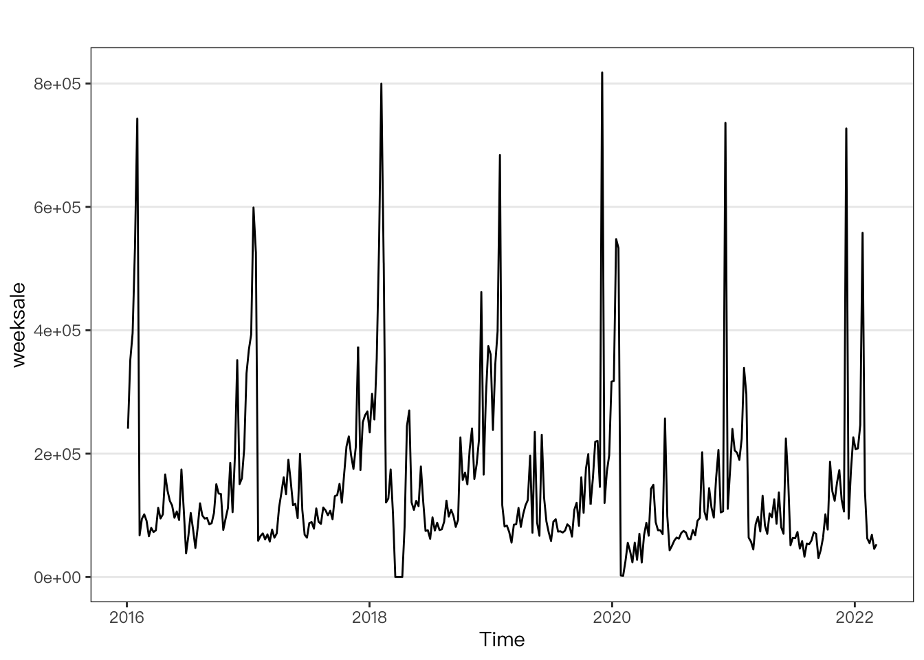
splits <- ts_split(weeksale, 8)
train <- splits$train
test <- splits$test
BATS/TBATS
For BATS Model,
\(\operatorname{BATS}\left(\omega, \phi, p, q, m_{1}, m_{2}, \ldots, m_{T}\right)\)
# bats model
bats_m <- bats(train)
bats_m
## BATS(0.354, {1,0}, -, {52})
##
## Call: bats(y = train)
##
## Parameters
## Lambda: 0.353777
## Alpha: 0.06931721
## Gamma Values: -0.2472086
## AR coefficients: 0.353693
##
## Seed States:
## [,1]
## [1,] 236.2172862
## [2,] 48.6153298
## [3,] 25.6318979
## [4,] 65.9402978
## [5,] 48.5353739
## [6,] 34.5740092
## [7,] 32.2362991
## [8,] 17.0571974
## [9,] 18.2687693
## [10,] 12.1147339
## [11,] 17.6131427
## [12,] -0.8316901
## [13,] -1.5229147
## [14,] 12.8711144
## [15,] -14.7505548
## [16,] -19.1669848
## [17,] -19.8997841
## [18,] -21.1926193
## [19,] -23.4601100
## [20,] -20.8589143
## [21,] -22.8231038
## [22,] -28.4857736
## [23,] -28.1033726
## [24,] -32.0859166
## [25,] -26.6846780
## [26,] -22.8513308
## [27,] -35.7280360
## [28,] -42.0967584
## [29,] -13.6621107
## [30,] 18.7225542
## [31,] 3.6108027
## [32,] -18.6830362
## [33,] -9.1773408
## [34,] -1.2862120
## [35,] -0.1671799
## [36,] 20.2180037
## [37,] 5.0885815
## [38,] -11.7724907
## [39,] -41.3620492
## [40,] -46.7859929
## [41,] -49.6365415
## [42,] -57.6488590
## [43,] -24.3202110
## [44,] -37.3709292
## [45,] -28.7887699
## [46,] -25.1689822
## [47,] 5.6126602
## [48,] 5.6972456
## [49,] 48.6994849
## [50,] 93.1440007
## [51,] 77.8410675
## [52,] 60.1611764
## [53,] 59.6051217
## [54,] 0.0000000
## attr(,"lambda")
## [1] 0.3537771
##
## Sigma: 30.79541
## AIC: 8780.338For TBATS Model,
\(\operatorname{TBATS}\left(\omega, \phi, p, q,\left\{m_{1}, k_{1}\right\},\left\{m_{2}, k_{2}\right\}, \ldots,\left\{m_{T}, k_{T}\right\}\right)\)
# tbats model
tbats_m <- tbats(train)
tbats_m
## TBATS(0.346, {0,1}, -, {<52.19,5>})
##
## Call: tbats(y = train)
##
## Parameters
## Lambda: 0.345914
## Alpha: 0.01716498
## Gamma-1 Values: -0.009315079
## Gamma-2 Values: 0.005982234
## MA coefficients: 0.343452
##
## Seed States:
## [,1]
## [1,] 177.5373756
## [2,] 29.6240539
## [3,] 17.7008739
## [4,] 16.6389904
## [5,] 0.5296389
## [6,] -0.3902185
## [7,] -11.3794443
## [8,] -17.1882094
## [9,] 7.1278290
## [10,] 8.5281331
## [11,] 2.5042501
## [12,] 0.0000000
## attr(,"lambda")
## [1] 0.3459141
##
## Sigma: 31.59406
## AIC: 8771.571Check the KEY Difference!
Note that:
TBATS: The seed state for seasonal is \(2 \cdot k_1 = 2 \cdot 5 = 10\).
BATS: The seed state for seasonal is \(52\)! Much larger than TBATS
Performance
Compare Accuracy:
bats_fc <- forecast(bats_m, h = length(test))
tbats_fc <- forecast(tbats_m, h = length(test))

accuracy(bats_fc, test)
## ME RMSE MAE MPE MAPE MASE
## Training set 1199.837 89752.11 46368.39 -28256.17129 28276.14207 0.6546733
## Test set 5425.741 151518.01 92546.58 -41.36154 58.91754 1.3066612
## ACF1 Theil's U
## Training set -0.1925466 NA
## Test set -0.2937480 1.204268accuracy(tbats_fc, test)## ME RMSE MAE MPE MAPE MASE
## Training set 6471.137 99574.55 51738.22 -50245.07151 50265.01625 0.7304897
## Test set 36719.289 136648.52 68088.57 -15.87087 36.99544 0.9613396
## ACF1 Theil's U
## Training set -0.09246037 NA
## Test set 0.03653672 1.050218plots:
bats_cv <- tssv_direct(weeksale, test_horizon = 8, forecast_model = bats_forecast)

tbats_cv <- tssv_direct(weeksale, test_horizon = 8, forecast_model = tbats_forecast)

plot_tssv(bats_cv, max_hist = 52) +
  labs(title = "BSTS 8-step Forecast for weeksale data")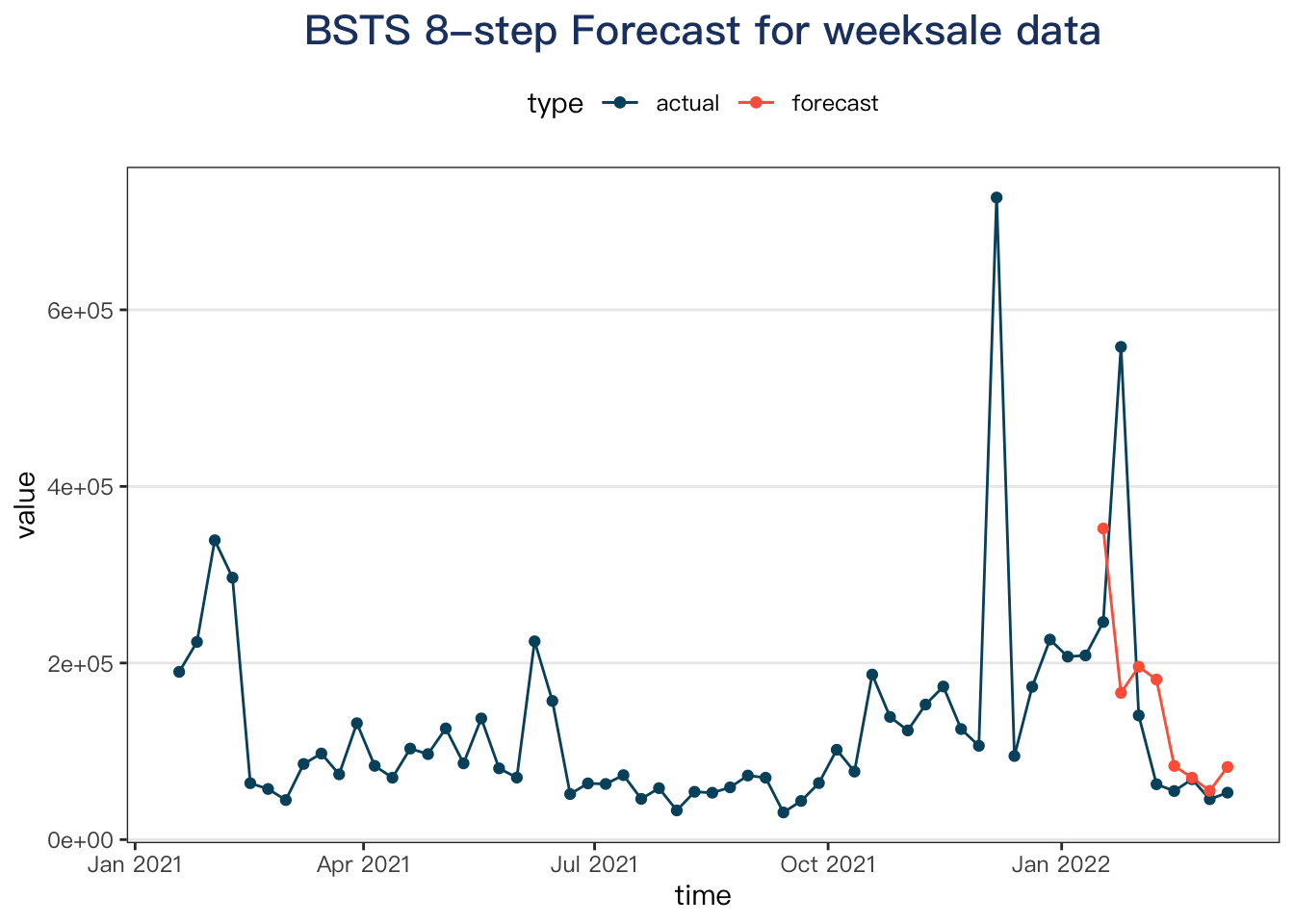
plot_tssv(tbats_cv, max_hist = 52) +
  labs(title = "TBSTS 8-step Forecast for weeksale data")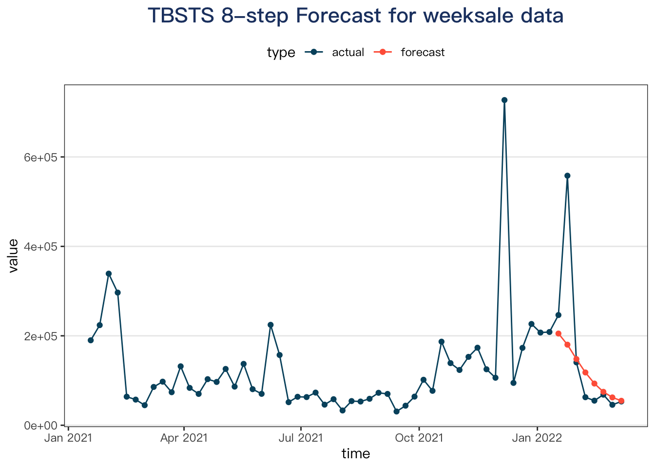
Here, the tbats model does a better job in terms of RMSE criteria.