Tidymodels Ecosystem Tutorial
Tiydmodels Ecosystem
I also hold this post on this RPub tutorial.
Introduction
First we should get a feeling of tidymodels ecosystem, and understand
what each package does!

Note that:
-
Data Resampling and Feature Engineering:
rsample,recipes -
Model Fitting and Tuning:
parsnip,tune,dials -
Model Evaluation:
yardstick
Big Picture
We will focus on the following packages although there are many more in the tidymodels ecosystem:
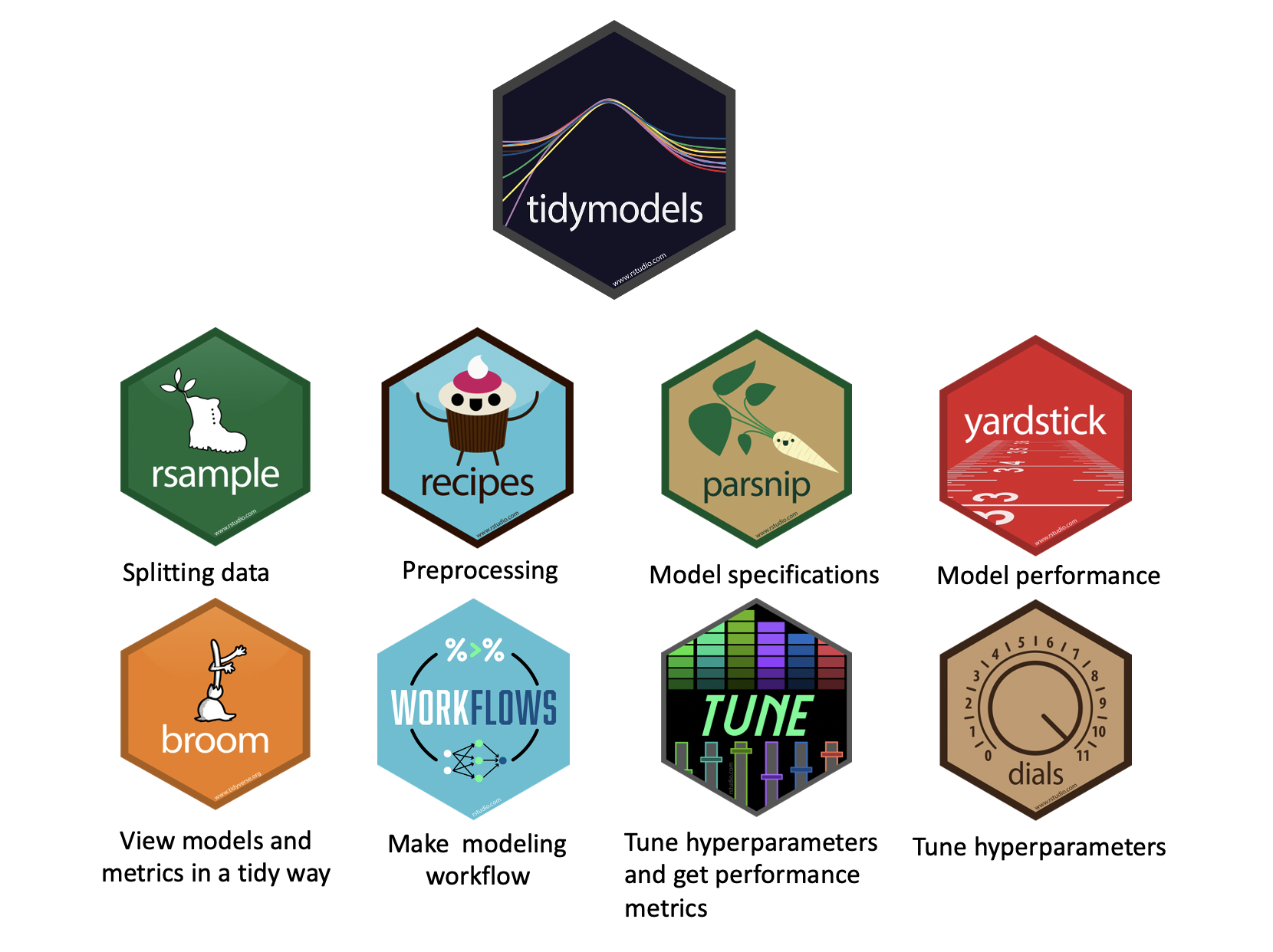
rsamples- to split the data into training and testing sets (as well as cross validation sets - more on that later!)recipes- to prepare the data with preprocessing (assign variables and preprocessing steps)parsnip- to specify and fit the data to a modelyardstickandtune- to evaluate model performanceworkflows- combining recipe and parsnip objects into a workflow (this makes it easier to keep track of what you have done and it makes it easier to modify specific steps)tuneanddials- model optimization (more on what hyperparameters are later too!)broom- to make the output from fitting a model easier to read
Here you can see a visual of how these packages work together in the process of performing a machine learning analysis:
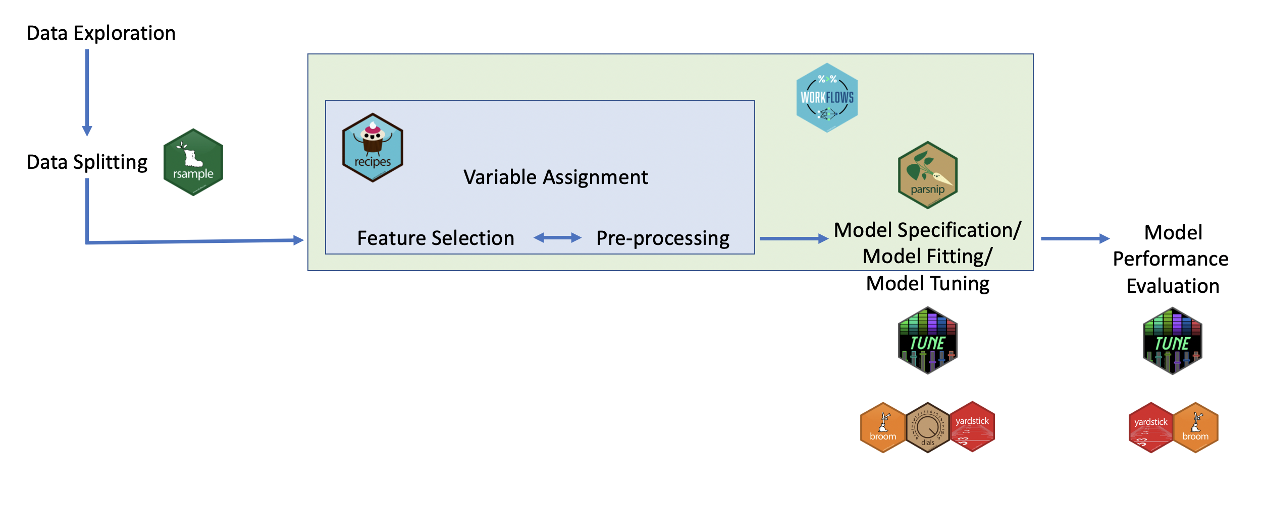
To illustrate how to use each of these packages, we will work through some examples.
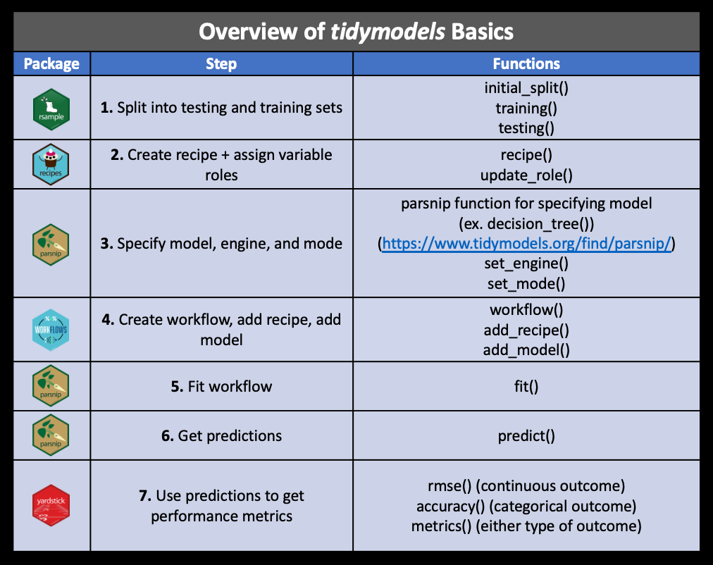
These are the major steps that we will cover in addition to some more advanced methods:
Other tidymodels packages include:
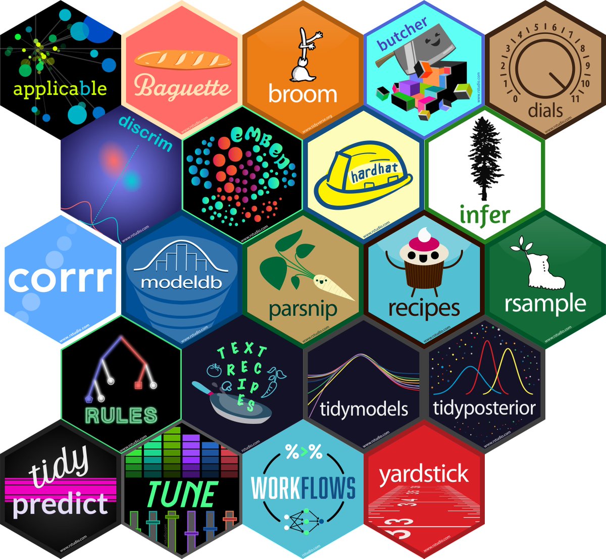
[source]
applicablecompares new data points with the training data to see how much the new data points appear to be an extrapolation of the training databaguetteis for speeding up bagging pipelinesbutcheris for dealing with pipelines that create model objects that take up too much memorydiscrimhas more model options for classificationembedhas extra preprocessing options for categorical predictorshardhathelps you to make new modeling packagescorrrhas more options for looking at correlation matricesruleshas more model options for prediction rule ensemblestext recipeshas extra preprocessing options for using text datatidypredictis for running predictions inside SQL databasesmodeldbis also for working within SQL databases and it allows fordplyrandtidyevaluse within a databasetidyposteriorcompares models using resampling statistics
Most of these packages offer advanced modeling options and we will not be covering how to use them.
Machine Learning with Tidymodels
Note that the data, code and other materials are from Chen Xing’s Modeling with Tidymodels in R lectureNotes.
library(tidymodels)
library(tidyverse)
zetaEDA::enable_zeta_ggplot_theme()

## this below is for copy button in html code chunk
## ignore it if not need

## remotes::install_github("rlesur/klippy")
klippy::klippy(position = "right")
rsample: Creating training and test datasets
The goal is to learn rsample pacakge!
Thersamplepackage is designed to create training and test datasets.
Creating a test dataset is important for estimating how a trained model will likely perform on new data. It also guards against overfitting, where a model memorizes patterns that exist only in the training data and performs poorly on new data.
home_sales data contains information on homes sold in the Seattle,
Washington area between 2015 and 2016.
The outcome variable in this data is selling_price.
home_sales <- read_rds("data/home_sales.rds")
head(home_sales)
## # A tibble: 6 × 8
##   selling_price home_age bedrooms bathrooms sqft_living sqft_lot sqft_basement
##           <dbl>    <dbl>    <dbl>     <dbl>       <dbl>    <dbl>         <dbl>
## 1        487000       10        4      2.5         2540     5001             0
## 2        465000       10        3      2.25        1530     1245           480
## 3        411000       18        2      2           1130     1148           330
## 4        635000        4        3      2.5         3350     4007           800
## 5        380000       24        5      2.5         2130     8428             0
## 6        495000       21        3      3.5         1650     1577           550
## # … with 1 more variable: floors <dbl>
Generate training and testing data set.
Note that:
strataarg ininitial_split()ensure that the random split with similar distribution of response variable.
?initial_split()

## Create a data split object
home_split <- initial_split(
  home_sales,
  prop = 0.7,
  ## stratification by outcome variable
  strata = selling_price
)

## Create the training data
home_training <- home_split %>%
  training()

## Create the test data
home_test <- home_split %>%
  testing()

## Check number of rows in each dataset
nrow(home_training)
## [1] 1042
nrow(home_test)
## [1] 450
Random sampling 得到的 training and testing set, distribution 是否一致呢?
## for training
home_training %>%
  summarize(across(selling_price, list(
    min = min,
    max = max,
    mean = mean,
    sd = sd
  )))
## # A tibble: 1 × 4
##   selling_price_min selling_price_max selling_price_mean selling_price_sd
##               <dbl>             <dbl>              <dbl>            <dbl>
## 1            350000            650000            478948.           80507.
## for testing
home_test %>%
  summarize(across(selling_price, list(
    min = min,
    max = max,
    mean = mean,
    sd = sd
  )))
## # A tibble: 1 × 4
##   selling_price_min selling_price_max selling_price_mean selling_price_sd
##               <dbl>             <dbl>              <dbl>            <dbl>
## 1            350000            650000            479401.           82151.
## note:
## Stratifying by the outcome variable ensures the model fitting process is performed on a representative sample of the original data.
distribution are quite similar!
parsnip: Fitting a linear regression model
The goal is to learn
parsnippackage!
Using parsnip to fit the model
## model setup
lm_mod <- linear_reg() %>%
  set_engine("lm") %>%
  set_mode("regression")

## check
lm_mod
## Linear Regression Model Specification (regression)
##
## Computational engine: lm
model specification
- {tidymodels}/{parsnip} Philosophy is to unify & make interfaces more predictable.
- Specify model type (e.g. linear regression, random forest …)
linear_reg()rand_forest()
- Specify engine (i.e. package implementation of algorithm)
set_engine("some package's implementation")
- declare mode (e.g. classification vs linear regression)
- use this when model can do both classification & regression
set_mode("regression")set_mode("classification")
- Specify model type (e.g. linear regression, random forest …)
Modeling functions in parsnip separate model arguments into two categories:
-
Main arguments are more commonly used and tend to be available across engines.
-
Engine arguments are either specific to a particular engine or used more rarely.
Note:
-
一般来说,
set_engine()里面的参数就是包的名字,或者说给定包对应的主函数,例如:"lm"。如果要修改这个主函数的默认参数,也在set_engine()里修改,使用的是set_engine(...)的功能。 -
如果要修改某个方法的通用参数,(所谓通用参数,就是说这个参数和你用哪个包是无关的),那么在specify model type 的函数里给定,例如:
rand_forest(trees = 1000, min_n = 5)
Fitting model
lm_fit <- lm_mod %>%
  fit(selling_price ~ home_age + sqft_living, data = home_training)

## check
lm_fit
## parsnip model object
##
##
## Call:
## stats::lm(formula = selling_price ~ home_age + sqft_living, data = data)
##
## Coefficients:
## (Intercept)     home_age  sqft_living
##    290498.6      -1609.4        103.9
Obtain the estimated parameters
tidy(lm_fit)
## # A tibble: 3 × 5
##   term        estimate std.error statistic   p.value
##   <chr>          <dbl>     <dbl>     <dbl>     <dbl>
## 1 (Intercept)  290868.   7592.       38.3  6.10e-201
## 2 home_age      -1452.    173.       -8.40 1.49e- 16
## 3 sqft_living     103.      2.74     37.7  1.75e-196
Generate predictions
## using fitting model to get prediction
lm_pred <- lm_fit %>%
  predict(new_data = home_test)

head(lm_pred)
## # A tibble: 6 × 1
##     .pred
##     <dbl>
## 1 538413.
## 2 433433.
## 3 378981.
## 4 428202.
## 5 408554.
## 6 530970.
bind result
home_test_res <- home_test %>%
  select(selling_price, sqft_living, home_age) %>%
  bind_cols(lm_pred)

head(home_test_res)
## # A tibble: 6 × 4
##   selling_price sqft_living home_age   .pred
##           <dbl>       <dbl>    <dbl>   <dbl>
## 1        495000        1650       21 430724.
## 2        425000        1920       11 473124.
## 3        495000        2140        3 507457.
## 4        559900        2930       20 564331.
## 5        552321        1960       29 451111.
## 6        525000        2450       28 503154.
yardstick: Evalucate Model Performance
The goal is to learn
yardstickpackage!
Input to yardstick functions:
all yardstick functions requires a tibble with columns:
-
true outcome (实际值)
-
model predictions,
.pred, (预测值)
For RMSE and R^2,
## calculate RMSE
home_test_res %>%
  rmse(truth = selling_price, estimate = .pred)
## # A tibble: 1 × 3
##   .metric .estimator .estimate
##   <chr>   <chr>          <dbl>
## 1 rmse    standard      47624.
## calculate R^2
home_test_res %>%
  rsq(truth = selling_price, estimate = .pred)
## # A tibble: 1 × 3
##   .metric .estimator .estimate
##   <chr>   <chr>          <dbl>
## 1 rsq     standard       0.646
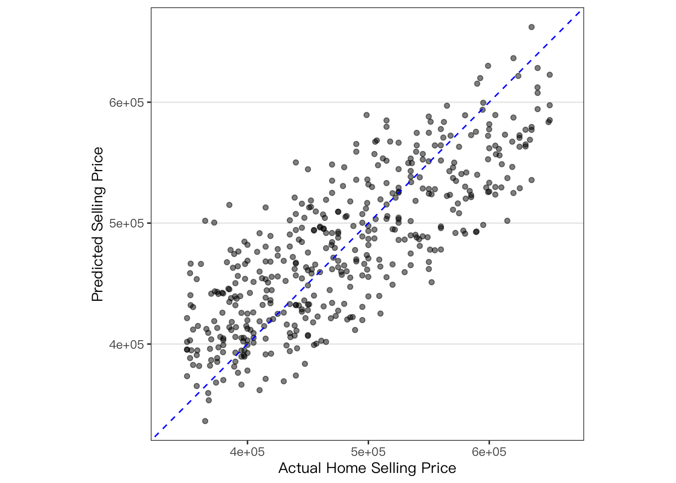
Visualize \(R^2\) plot:
coord_obs_pred() can be used in a ggplot to make the x- and y-axes
have the same exact scale along with an aspect ratio of one.
?coord_obs_pred
## note that the `coord_obs_pred` is from `tune` pacakge!
home_test_res %>%
  ggplot(aes(x = selling_price, y = .pred)) +
  geom_point(alpha = .5) +
  geom_abline(color = "blue", linetype = 2) +
  coord_obs_pred() +
  labs(x = "Actual Home Selling Price", y = "Predicted Selling Price")
Streamlining Model Fitting
?last_fit()
last_fit() takes a model specification, model formula, and data split
object Performs the following:
-
Creates training and test datasets
-
Fits the model to the training data
-
Calculates metrics and predictions on the test data
-
Returns an object with all results
## define linear regression model
lm_mod <- linear_reg() %>%
  set_engine("lm") %>%
  set_mode("regression")

## Train linear_model with last_fit()
lm_fit <- lm_mod %>%
  last_fit(selling_price ~ ., split = home_split)

## check
lm_fit
## # Resampling results
## # Manual resampling
## # A tibble: 1 × 6
##   splits             id               .metrics .notes   .predictions .workflow
##   <list>             <chr>            <list>   <list>   <list>       <list>
## 1 <split [1042/450]> train/test split <tibble> <tibble> <tibble>     <workflow>
Collect predictions and view results
?tune::collect_predictions()

## Collect predictions and view results
predictions_df <- lm_fit %>% collect_predictions()

## check
head(predictions_df)
## # A tibble: 6 × 5
##   id                 .pred  .row selling_price .config
##   <chr>              <dbl> <int>         <dbl> <chr>
## 1 train/test split 527930.     1        487000 Preprocessor1_Model1
## 2 train/test split 424149.     2        465000 Preprocessor1_Model1
## 3 train/test split 399071.     3        411000 Preprocessor1_Model1
## 4 train/test split 438494.     6        495000 Preprocessor1_Model1
## 5 train/test split 400976.     7        355000 Preprocessor1_Model1
## 6 train/test split 478599.    10        535000 Preprocessor1_Model1
Question: when should I use
last_fit()function?
After carefully reading the help file of the last_fit() function, the answer is obvious.
当我们尝试拟合了不同的模型,以及完成了hyper-parameter tuning,从而找到了最满意的模型。那么最后一步就是将这个模型重新在training set上拟合一遍,然后看看它在testing set 上的表现情况。
last_fit() 的目的就是帮助我们完成这最后的一步!
Classification Models
We will be working with the telecom_df dataset which contains
information on customers of a telecommunications company. The outcome
variable is canceled_service and it records whether a customer
canceled their contract with the company. The predictor variables
contain information about customers’ cell phone and internet usage as
well as their contract type and monthly charges.
telecom_df <- read_rds("data/telecom_df.rds")

## check
head(telecom_df)
## # A tibble: 6 × 9
##   canceled_service cellular_service avg_data_gb avg_call_mins avg_intl_mins
##   <fct>            <fct>                  <dbl>         <dbl>         <dbl>
## 1 yes              single_line             7.78           497           127
## 2 yes              single_line             9.04           336            88
## 3 no               single_line            10.3            262            55
## 4 yes              multiple_lines          5.08           250           107
## 5 no               multiple_lines          8.05           328           122
## 6 no               single_line             9.3            326           114
## # … with 4 more variables: internet_service <fct>, contract <fct>,
## #   months_with_company <dbl>, monthly_charges <dbl>
Train/Test Set
Using rsample package again to create training and testing sets.
telecom_split <- initial_split(
  data = telecom_df,
  prop = .75,
  strata = canceled_service
)

## for training
telecom_training <- telecom_split %>%
  training()

## for testing
telecom_test <- telecom_split %>%
  testing()

## check
nrow(telecom_training)
## [1] 731
nrow(telecom_test)
## [1] 244
Model Fitting
Using parsnip package to fit a logistic regression model,
## Specify a logistic regression model
logistic_model <- logistic_reg() %>%
  ## Set the engine
  set_engine("glm") %>%
  ## Set the mode
  set_mode("classification")

## Fit to training data
logistic_fit <- logistic_model %>%
  fit(
    canceled_service ~ avg_call_mins + avg_intl_mins + monthly_charges,
    data = telecom_training
  )

## Print model fit object
logistic_fit
## parsnip model object
##
##
## Call:  stats::glm(formula = canceled_service ~ avg_call_mins + avg_intl_mins +
##     monthly_charges, family = stats::binomial, data = data)
##
## Coefficients:
##     (Intercept)    avg_call_mins    avg_intl_mins  monthly_charges
##        2.607512        -0.011708         0.023125        -0.002036
##
## Degrees of Freedom: 730 Total (i.e. Null);  727 Residual
## Null Deviance:       932.4
## Residual Deviance: 794.2     AIC: 802.2
Generate Prediction
## Predict outcome categories
class_preds <- predict(
  logistic_fit,
  new_data = telecom_test,
  type = "class"
)

## Obtain estimated probabilities for each outcome value
prob_preds <- predict(
  logistic_fit,
  new_data = telecom_test,
  type = "prob"
)

## Combine test set results
telecom_results <- telecom_test %>%
  select(canceled_service) %>%
  bind_cols(class_preds, prob_preds)

## View results tibble
telecom_results %>%
  head()
## # A tibble: 6 × 4
##   canceled_service .pred_class .pred_yes .pred_no
##   <fct>            <fct>           <dbl>    <dbl>
## 1 no               no              0.354    0.646
## 2 no               no              0.226    0.774
## 3 yes              yes             0.813    0.187
## 4 yes              yes             0.539    0.461
## 5 yes              yes             0.583    0.417
## 6 yes              no              0.152    0.848
Assessing Model Fitting
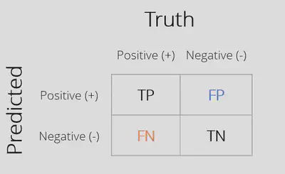
Confusion Matrix: Matrix with counts of all combinations of actual and predicted outcome values.
Correct Predictions
-
True Positive (TP)
-
True Negative (TN)
Classification Errors
-
False Positive (FP)
-
False Negative (FN)
## Calculate the confusion matrix
yardstick::conf_mat(
  telecom_results,
  truth = canceled_service,
  estimate = .pred_class
)
##           Truth
## Prediction yes  no
##        yes  37  25
##        no   45 137
Some Metrics:
-
\(accuracy = \frac{TP + TN}{TP + FP + TN + FN}\), is classification accuracy. -
\(sensitivity = \frac{TP}{TP + FP}\), is the proportion of all positive cases that were correctly classified. -
\(specificity = \frac{TN}{TN + FN}\), is the proportion of all negative cases that were correctly classified. -
\(false \ positive \ rate\ (FPR) \ = 1 - specificity\), is the proportion of false positives among true negatives.
## Calculate the accuracy
yardstick::accuracy(
  telecom_results,
  truth = canceled_service,
  estimate = .pred_class
)
## # A tibble: 1 × 3
##   .metric  .estimator .estimate
##   <chr>    <chr>          <dbl>
## 1 accuracy binary         0.713
## Calculate the sensitivity
yardstick::sens(
  telecom_results,
  truth = canceled_service,
  estimate = .pred_class
)
## # A tibble: 1 × 3
##   .metric .estimator .estimate
##   <chr>   <chr>          <dbl>
## 1 sens    binary         0.451
## Calculate the specificity
yardstick::spec(
  telecom_results,
  truth = canceled_service,
  estimate = .pred_class
)
## # A tibble: 1 × 3
##   .metric .estimator .estimate
##   <chr>   <chr>          <dbl>
## 1 spec    binary         0.846
Instead of calculating accuracy, sensitivity, and specificity separately, you can create your own metric function that calculates all three at the same time.
## Create a custom metric function
telecom_metrics <- metric_set(
  yardstick::accuracy,
  yardstick::sens,
  yardstick::spec
)

## Calculate metrics using model results tibble
telecom_metrics(
  telecom_results,
  truth = canceled_service,
  estimate = .pred_class
)
## # A tibble: 3 × 3
##   .metric  .estimator .estimate
##   <chr>    <chr>          <dbl>
## 1 accuracy binary         0.713
## 2 sens     binary         0.451
## 3 spec     binary         0.846
Calculate Many metrics all together,
## Create a confusion matrix
conf_mat(
  telecom_results,
  truth = canceled_service,
  estimate = .pred_class
) %>%
  ## Pass to the summary() function
  summary()
## # A tibble: 13 × 3
##    .metric              .estimator .estimate
##    <chr>                <chr>          <dbl>
##  1 accuracy             binary         0.713
##  2 kap                  binary         0.316
##  3 sens                 binary         0.451
##  4 spec                 binary         0.846
##  5 ppv                  binary         0.597
##  6 npv                  binary         0.753
##  7 mcc                  binary         0.322
##  8 j_index              binary         0.297
##  9 bal_accuracy         binary         0.648
## 10 detection_prevalence binary         0.254
## 11 precision            binary         0.597
## 12 recall               binary         0.451
## 13 f_meas               binary         0.514
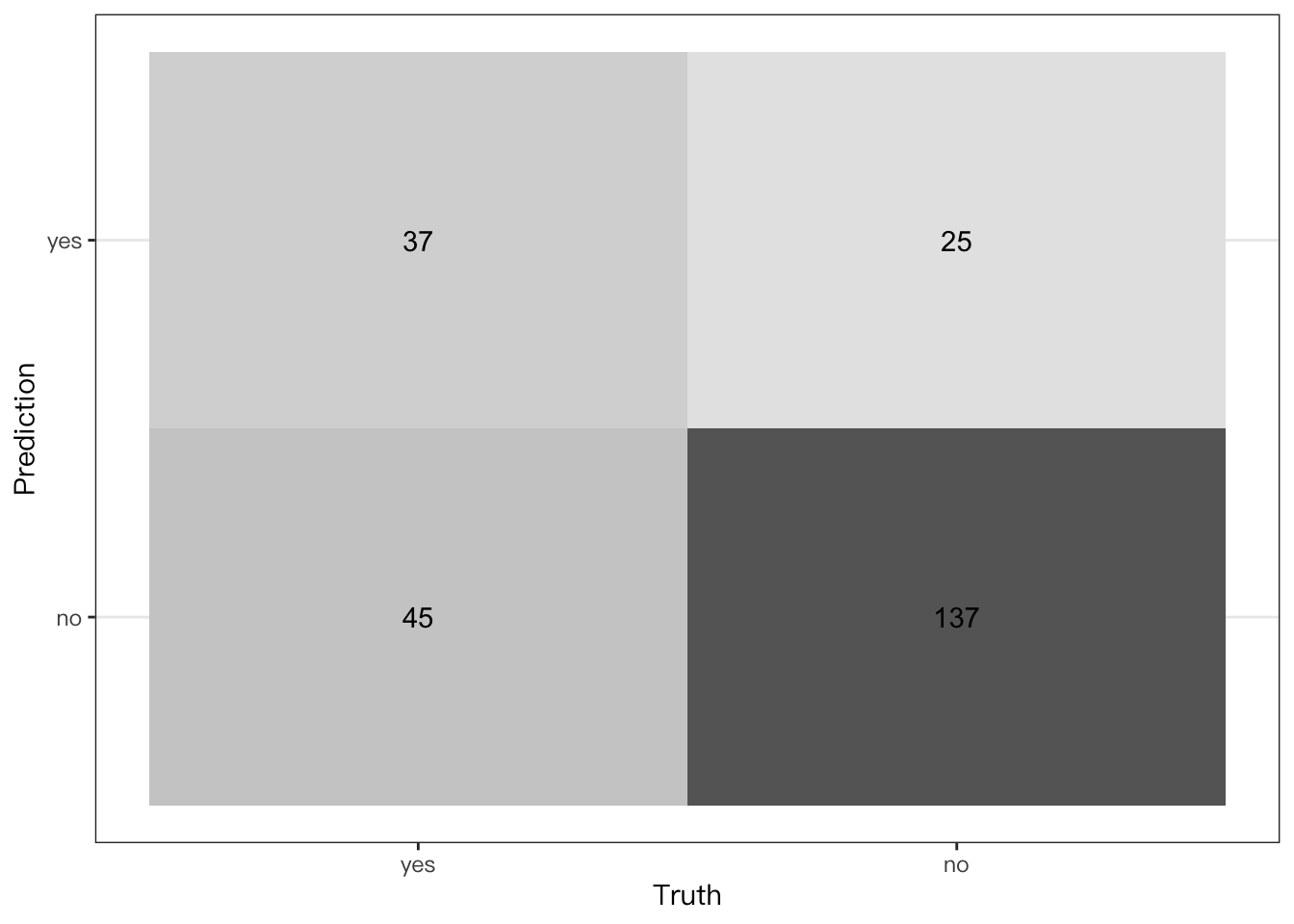
Visualize Model Performance
Plotting a confusion matrix,
conf_mat(
  telecom_results,
  truth = canceled_service,
  estimate = .pred_class
) %>%
  ## Create a heat map
  autoplot(type = "heatmap")
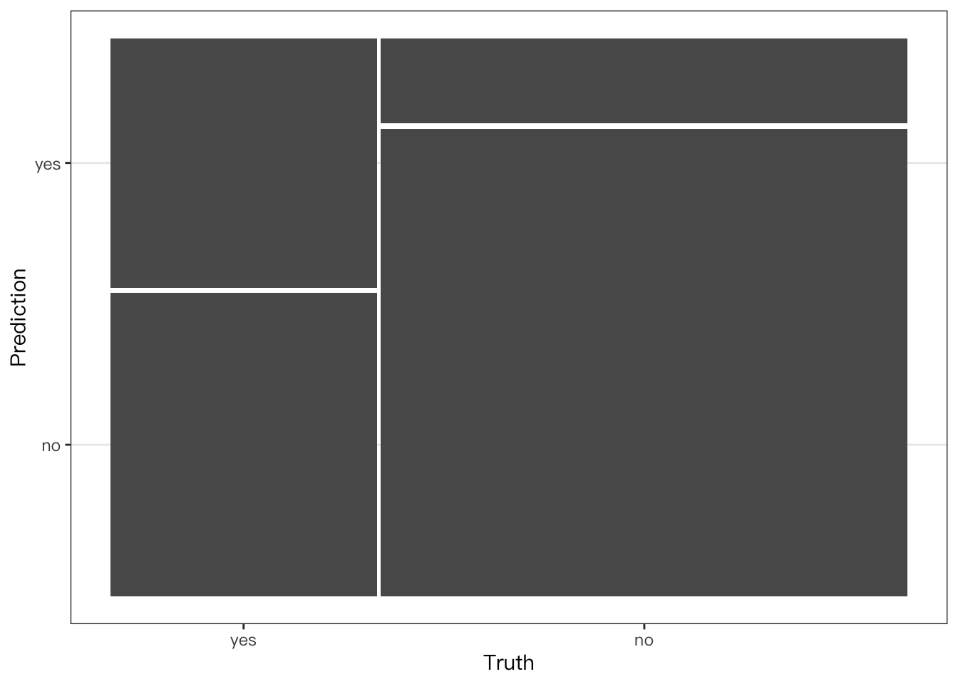
conf_mat(
  telecom_results,
  truth = canceled_service,
  estimate = .pred_class
) %>%
  ## Create a mosaic map
  autoplot(type = "mosaic")
ROC curves and area under the ROC curve
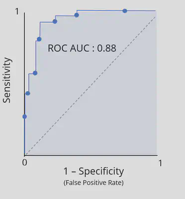
Summarizing the ROC curve
The area under the ROC curve (ROC AUC) captures the ROC curve information of a classi,cation model in a single number
Useful interpretation as a le2er grade of classifcation performance
-
A - [0.9, 1
-
B - [0.8, 0.9)
-
C - [0.7, 0.8)
-
D - [0.6, 0.7)
-
F - [0.5, 0.6)
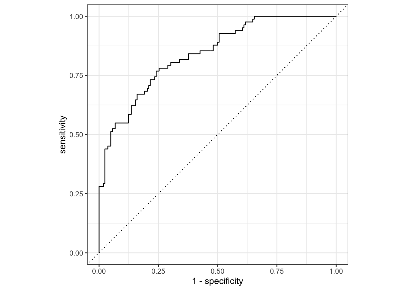
## Plot ROC curve
telecom_results %>%
  ## Calculate metrics across thresholds
  roc_curve(
    truth = canceled_service,
    estimate = .pred_yes
  ) %>%
  autoplot()
## Calculate the ROC AUC
telecom_results %>%
  roc_auc(
    truth = canceled_service,
    estimate = .pred_yes
  )
## # A tibble: 1 × 3
##   .metric .estimator .estimate
##   <chr>   <chr>          <dbl>
## 1 roc_auc binary         0.713
Automatic Tidymodels Workflow
## Train model with last_fit()
telecom_last_fit <- logistic_model %>%
  last_fit(
    ## formula
    canceled_service ~ avg_call_mins + avg_intl_mins + monthly_charges,
    split = telecom_split
  )

## View test set metrics
telecom_last_fit %>%
  collect_metrics()
## # A tibble: 2 × 4
##   .metric  .estimator .estimate .config
##   <chr>    <chr>          <dbl> <chr>
## 1 accuracy binary         0.713 Preprocessor1_Model1
## 2 roc_auc  binary         0.713 Preprocessor1_Model1
## Collect predictions
last_fit_results <- telecom_last_fit %>%
  collect_predictions()

## View results
last_fit_results %>%
  head()
## # A tibble: 6 × 7
##   id               .pred_yes .pred_no  .row .pred_class canceled_service .config
##   <chr>                <dbl>    <dbl> <int> <fct>       <fct>            <chr>
## 1 train/test split     0.354    0.646     3 no          no               Prepro…
## 2 train/test split     0.226    0.774     6 no          no               Prepro…
## 3 train/test split     0.813    0.187     7 yes         yes              Prepro…
## 4 train/test split     0.539    0.461     9 yes         yes              Prepro…
## 5 train/test split     0.583    0.417    12 yes         yes              Prepro…
## 6 train/test split     0.152    0.848    14 no          yes              Prepro…
## Custom metrics function
last_fit_metrics <- metric_set(
  yardstick::accuracy,
  yardstick::sens,
  yardstick::spec,
  yardstick::roc_auc
)

## Calculate metrics
last_fit_metrics(
  last_fit_results,
  truth = canceled_service,
  estimate = .pred_class,
  ## note that roc_auc needs predicted probability
  .pred_yes
)
## # A tibble: 4 × 3
##   .metric  .estimator .estimate
##   <chr>    <chr>          <dbl>
## 1 accuracy binary         0.713
## 2 sens     binary         0.451
## 3 spec     binary         0.846
## 4 roc_auc  binary         0.713
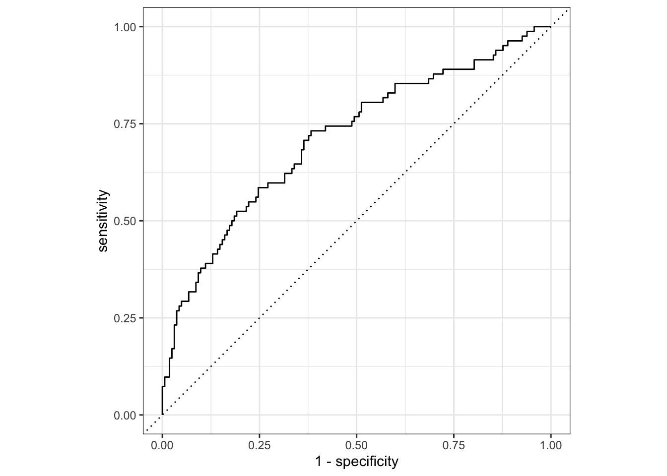
Now let’s try if we can improved the model by add one more regressor.
## new fitted model
new_fit <- logistic_model %>%
  last_fit(
    canceled_service ~ avg_call_mins + avg_intl_mins + monthly_charges + months_with_company,
    split = telecom_split
  )

## collection metrics, the accuracy and roc_auc indeed improved
new_fit %>%
  collect_metrics()
## # A tibble: 2 × 4
##   .metric  .estimator .estimate .config
##   <chr>    <chr>          <dbl> <chr>
## 1 accuracy binary         0.803 Preprocessor1_Model1
## 2 roc_auc  binary         0.827 Preprocessor1_Model1
## collection predictions
new_pred <- new_fit %>%
  collect_predictions()

## check ROC curve
new_pred %>%
  roc_curve(truth = canceled_service, estimate = .pred_yes) %>%
  autoplot()
Feature Engineering
Goal is to learn
recipepacakge.
-
step 1: Specify variables,
recipe(y ~ a+ b + …, data = dat) -
step 2: Define pre-precessing steps,
step_*() -
step 3: Provide dataset(s) for recipe steps,
prep() -
step 4: Apply Pre-precessing,
bake()
Creating recipe objects
The first step in feature engineering is to specify a recipeobject
with the recipe() function and add data preprocessing steps with one
or more step_*() functions. Storing all of this information in a
single recipe object makes it easier to manage complex feature
engineering pipelines and transform new data sources.
## Specify feature engineering recipe
telecom_log_rec <- recipe(
  ## define the response variable
  canceled_service ~ .,
  data = telecom_training
) %>%
  ## Add log transformation step
  step_log(avg_call_mins, avg_intl_mins, base = 10)

## View variable roles and data types
telecom_log_rec %>%
  summary()
## # A tibble: 9 × 4
##   variable            type    role      source
##   <chr>               <chr>   <chr>     <chr>
## 1 cellular_service    nominal predictor original
## 2 avg_data_gb         numeric predictor original
## 3 avg_call_mins       numeric predictor original
## 4 avg_intl_mins       numeric predictor original
## 5 internet_service    nominal predictor original
## 6 contract            nominal predictor original
## 7 months_with_company numeric predictor original
## 8 monthly_charges     numeric predictor original
## 9 canceled_service    nominal outcome   original
The next step in the feature engineering process is to train your recipe object using the training data. Then you will be able to apply your trained recipe to both the training and test datasets in order to prepare them for use in model fitting and model evaluation.
## Train the telecom_log_rec object
telecom_log_rec_prep <- telecom_log_rec %>%
  prep(training = telecom_training)

## View results
telecom_log_rec_prep
## Recipe
##
## Inputs:
##
##       role #variables
##    outcome          1
##  predictor          8
##
## Training data contained 731 data points and no missing data.
##
## Operations:
##
## Log transformation on avg_call_mins, avg_intl_mins [trained]
## apply pre-processing on training set
telecom_log_rec_prep %>%
  bake(new_data = NULL)
## # A tibble: 731 × 9
##    cellular_service avg_data_gb avg_call_mins avg_intl_mins internet_service
##    <fct>                  <dbl>         <dbl>         <dbl> <fct>
##  1 multiple_lines          8.05          2.52          2.09 digital
##  2 multiple_lines          9.4           2.49          2.17 fiber_optic
##  3 multiple_lines          9.96          2.53          2.13 fiber_optic
##  4 multiple_lines         10.2           2.60          2.06 fiber_optic
##  5 single_line             6.69          2.55          1.96 digital
##  6 multiple_lines          4.11          2.57          1.81 digital
##  7 multiple_lines          5.17          2.53          2.08 digital
##  8 single_line             8.67          1.97          2.12 fiber_optic
##  9 multiple_lines          9.24          2.59          2.15 fiber_optic
## 10 multiple_lines         11.0           2.59          1.89 fiber_optic
## # … with 721 more rows, and 4 more variables: contract <fct>,
## #   months_with_company <dbl>, monthly_charges <dbl>, canceled_service <fct>
## apply pre-processing on testing set
telecom_log_rec_prep %>%
  bake(new_data = telecom_test)
## # A tibble: 244 × 9
##    cellular_service avg_data_gb avg_call_mins avg_intl_mins internet_service
##    <fct>                  <dbl>         <dbl>         <dbl> <fct>
##  1 single_line            10.3           2.42          1.74 fiber_optic
##  2 single_line             9.3           2.51          2.06 fiber_optic
##  3 multiple_lines          8.01          2.72          1.99 fiber_optic
##  4 single_line             5.29          2.62          1.98 digital
##  5 single_line             6.23          2.63          1.98 fiber_optic
##  6 single_line             7.07          2.40          1.97 fiber_optic
##  7 single_line             9.37          2.58          1.94 fiber_optic
##  8 multiple_lines         10.6           2.45          2.17 fiber_optic
##  9 multiple_lines          7.86          2.58          2.21 digital
## 10 single_line             8.04          2.46          1.67 fiber_optic
## # … with 234 more rows, and 4 more variables: contract <fct>,
## #   months_with_company <dbl>, monthly_charges <dbl>, canceled_service <fct>
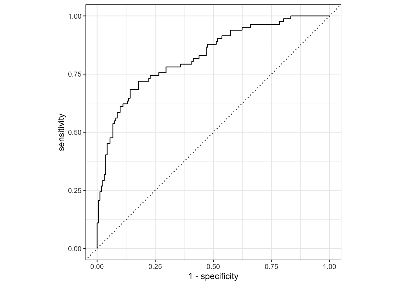
Numeric Predictors
Fix multicolinearity problems caused by highly correlated predictors.
telecom_training %>%
  select(where(is.numeric)) %>%
  cor()
##                     avg_data_gb avg_call_mins avg_intl_mins months_with_company
## avg_data_gb           1.0000000   0.195307838     0.1565105         0.386500807
## avg_call_mins         0.1953078   1.000000000     0.0737045         0.006322915
## avg_intl_mins         0.1565105   0.073704496     1.0000000         0.222895844
## months_with_company   0.3865008   0.006322915     0.2228958         1.000000000
## monthly_charges       0.9561583   0.189384250     0.1665923         0.407137668
##                     monthly_charges
## avg_data_gb               0.9561583
## avg_call_mins             0.1893842
## avg_intl_mins             0.1665923
## months_with_company       0.4071377
## monthly_charges           1.0000000
telecom_training %>%
  ggplot(aes(x = avg_data_gb, y = monthly_charges)) +
  geom_point() +
  labs(title = "Muticolinearity Example")
use
step_corr()and its argumentthreshold
Selecting predictors by type using:
-
all_outcomes(): Selects the outcome variable -
all_numeric(): Selects all numeric variables (could include outcome variable if it is numeric)
## Specify a recipe object
telecom_cor_rec <- recipe(
  ## define outcome variable
  canceled_service ~ .,
  data = telecom_training
) %>%
  ## Remove correlated variables
  step_corr(all_numeric_predictors(), threshold = 0.8)

## Train the recipe
telecom_cor_rec_prep <- telecom_cor_rec %>%
  prep(training = telecom_training)

## Apply to training data
telecom_cor_rec_prep %>%
  bake(new_data = NULL)
## # A tibble: 731 × 8
##    cellular_service avg_data_gb avg_call_mins avg_intl_mins internet_service
##    <fct>                  <dbl>         <dbl>         <dbl> <fct>
##  1 multiple_lines          8.05           328           122 digital
##  2 multiple_lines          9.4            312           147 fiber_optic
##  3 multiple_lines          9.96           340           136 fiber_optic
##  4 multiple_lines         10.2            402           116 fiber_optic
##  5 single_line             6.69           352            91 digital
##  6 multiple_lines          4.11           371            64 digital
##  7 multiple_lines          5.17           341           119 digital
##  8 single_line             8.67            93           131 fiber_optic
##  9 multiple_lines          9.24           392           142 fiber_optic
## 10 multiple_lines         11.0            390            78 fiber_optic
## # … with 721 more rows, and 3 more variables: contract <fct>,
## #   months_with_company <dbl>, canceled_service <fct>
## Apply to test data
telecom_cor_rec_prep %>%
  bake(new_data = telecom_test)
## # A tibble: 244 × 8
##    cellular_service avg_data_gb avg_call_mins avg_intl_mins internet_service
##    <fct>                  <dbl>         <dbl>         <dbl> <fct>
##  1 single_line            10.3            262            55 fiber_optic
##  2 single_line             9.3            326           114 fiber_optic
##  3 multiple_lines          8.01           525            97 fiber_optic
##  4 single_line             5.29           417            96 digital
##  5 single_line             6.23           429            96 fiber_optic
##  6 single_line             7.07           249            94 fiber_optic
##  7 single_line             9.37           382            87 fiber_optic
##  8 multiple_lines         10.6            281           147 fiber_optic
##  9 multiple_lines          7.86           378           164 digital
## 10 single_line             8.04           290            47 fiber_optic
## # … with 234 more rows, and 3 more variables: contract <fct>,
## #   months_with_company <dbl>, canceled_service <fct>
For Normalization calling
step_normalize
Normalization will center and scale numeric variable, i.e. subtract mean and divide by the standard deviation.
## Specify a recipe object
telecom_norm_rec <- recipe(
  canceled_service ~ .,
  data = telecom_training
) %>%
  ## Remove correlated variables
  step_corr(all_numeric(), threshold = 0.8) %>%
  ## Normalize numeric predictors
  step_normalize(all_numeric())

## Train the recipe
telecom_norm_rec_prep <- telecom_norm_rec %>%
  prep(training = telecom_training)

## Apply to test data
telecom_norm_rec_prep %>%
  bake(new_data = telecom_test)
## # A tibble: 244 × 8
##    cellular_service avg_data_gb avg_call_mins avg_intl_mins internet_service
##    <fct>                  <dbl>         <dbl>         <dbl> <fct>
##  1 single_line            1.08         -1.15         -1.73  fiber_optic
##  2 single_line            0.550        -0.300         0.206 fiber_optic
##  3 multiple_lines        -0.126         2.34         -0.352 fiber_optic
##  4 single_line           -1.55          0.906        -0.385 digital
##  5 single_line           -1.06          1.07         -0.385 fiber_optic
##  6 single_line           -0.619        -1.32         -0.450 fiber_optic
##  7 single_line            0.587         0.442        -0.680 fiber_optic
##  8 multiple_lines         1.26         -0.896         1.29  fiber_optic
##  9 multiple_lines        -0.205         0.389         1.84  digital
## 10 single_line           -0.111        -0.777        -1.99  fiber_optic
## # … with 234 more rows, and 3 more variables: contract <fct>,
## #   months_with_company <dbl>, canceled_service <fct>
Nominal Predictors
Dummy variable Encoding: Excludes one value from original set of data values, i.e. n distinct values produce (n-1) indictor variables.
use
step_dummy()function
Selecting columns by type: all_nominal()
## Create a recipe that predicts canceled_service using the training data
telecom_recipe <- recipe(
  canceled_service ~ .,
  data = telecom_training
) %>%
  ## Remove correlated predictors
  step_corr(all_numeric(), threshold = .8) %>%
  ## Normalize numeric predictors
  step_normalize(all_numeric()) %>%
  ## Create dummy variables
  step_dummy(all_nominal(), -all_outcomes())

## Train your recipe and apply it to the test data
telecom_recipe %>%
  prep(train = telecom_training) %>%
  bake(new_data = telecom_test)
## # A tibble: 244 × 9
##    avg_data_gb avg_call_mins avg_intl_mins months_with_company canceled_service
##          <dbl>         <dbl>         <dbl>               <dbl> <fct>
##  1       1.08         -1.15         -1.73               0.654  no
##  2       0.550        -0.300         0.206             -0.342  no
##  3      -0.126         2.34         -0.352             -0.581  yes
##  4      -1.55          0.906        -0.385             -1.02   yes
##  5      -1.06          1.07         -0.385             -0.0231 yes
##  6      -0.619        -1.32         -0.450             -0.581  yes
##  7       0.587         0.442        -0.680             -1.18   no
##  8       1.26         -0.896         1.29               0.813  no
##  9      -0.205         0.389         1.84              -0.421  no
## 10      -0.111        -0.777        -1.99               0.534  yes
## # … with 234 more rows, and 4 more variables:
## #   cellular_service_single_line <dbl>, internet_service_digital <dbl>,
## #   contract_one_year <dbl>, contract_two_year <dbl>
Complete Model Workflow
## 1. feature engineering-----------------------------------
telecom_recipe <- recipe(
  canceled_service ~ .,
  data = telecom_training
) %>%
  ## Removed correlated predictors
  step_corr(all_numeric(), threshold = 0.8) %>%
  ## Log transform numeric predictors
  step_log(all_numeric(), base = 10) %>%
  ## Normalize numeric predictors
  step_normalize(all_numeric()) %>%
  ## Create dummy variables
  step_dummy(all_nominal(), -all_outcomes())

## Train recipe
telecom_recipe_prep <- telecom_recipe %>%
  prep(training = telecom_training)

## Apply pre-processing recipe on training data
telecom_training_prep <- telecom_recipe_prep %>%
  bake(new_data = NULL)

## Apply pre-processing recipe on test data
telecom_test_prep <- telecom_recipe_prep %>%
  bake(new_data = telecom_test)

telecom_test_prep
## # A tibble: 244 × 9
##    avg_data_gb avg_call_mins avg_intl_mins months_with_company canceled_service
##          <dbl>         <dbl>         <dbl>               <dbl> <fct>
##  1     1.00           -1.06         -1.99              0.717   no
##  2     0.591          -0.165         0.323             0.207   no
##  3     0.00120         1.79         -0.190             0.00453 yes
##  4    -1.64            0.845        -0.223            -0.633   yes
##  5    -0.991           0.961        -0.223             0.411   yes
##  6    -0.492          -1.27         -0.290             0.00453 yes
##  7     0.620           0.485        -0.536            -1.14    no
##  8     1.13           -0.775         1.13              0.774   no
##  9    -0.0734          0.442         1.48              0.145   no
## 10     0.0160         -0.645        -2.49              0.672   yes
## # … with 234 more rows, and 4 more variables:
## #   cellular_service_single_line <dbl>, internet_service_digital <dbl>,
## #   contract_one_year <dbl>, contract_two_year <dbl>
## 2. Model Fitting-----------------------------------

## Train logistic model
logistic_fit <- logistic_model %>%
  fit(canceled_service ~ ., data = telecom_training_prep)

## Obtain class predictions
class_preds <- predict(
  logistic_fit,
  new_data = telecom_test_prep,
  type = "class"
)

## Obtain estimated probabilities
prob_preds <- predict(
  logistic_fit,
  new_data = telecom_test_prep,
  type = "prob"
)

## Combine test set results
telecom_results <- telecom_test_prep %>%
  select(canceled_service) %>%
  bind_cols(class_preds, prob_preds)

telecom_results
## # A tibble: 244 × 4
##    canceled_service .pred_class .pred_yes .pred_no
##    <fct>            <fct>           <dbl>    <dbl>
##  1 no               no             0.169     0.831
##  2 no               no             0.233     0.767
##  3 yes              yes            0.844     0.156
##  4 yes              no             0.379     0.621
##  5 yes              no             0.440     0.560
##  6 yes              no             0.153     0.847
##  7 no               yes            0.753     0.247
##  8 no               no             0.0197    0.980
##  9 no               no             0.0877    0.912
## 10 yes              no             0.422     0.578
## # … with 234 more rows
## 3. Model Performance Metric-----------------------------------

## Create a confusion matrix
telecom_results %>%
  yardstick::conf_mat(truth = canceled_service, estimate = .pred_class)
##           Truth
## Prediction yes  no
##        yes  45  19
##        no   37 143
## Calculate sensitivity
telecom_results %>%
  yardstick::sens(truth = canceled_service, estimate = .pred_class)
## # A tibble: 1 × 3
##   .metric .estimator .estimate
##   <chr>   <chr>          <dbl>
## 1 sens    binary         0.549
## Calculate specificity
telecom_results %>%
  yardstick::spec(truth = canceled_service, estimate = .pred_class)
## # A tibble: 1 × 3
##   .metric .estimator .estimate
##   <chr>   <chr>          <dbl>
## 1 spec    binary         0.883
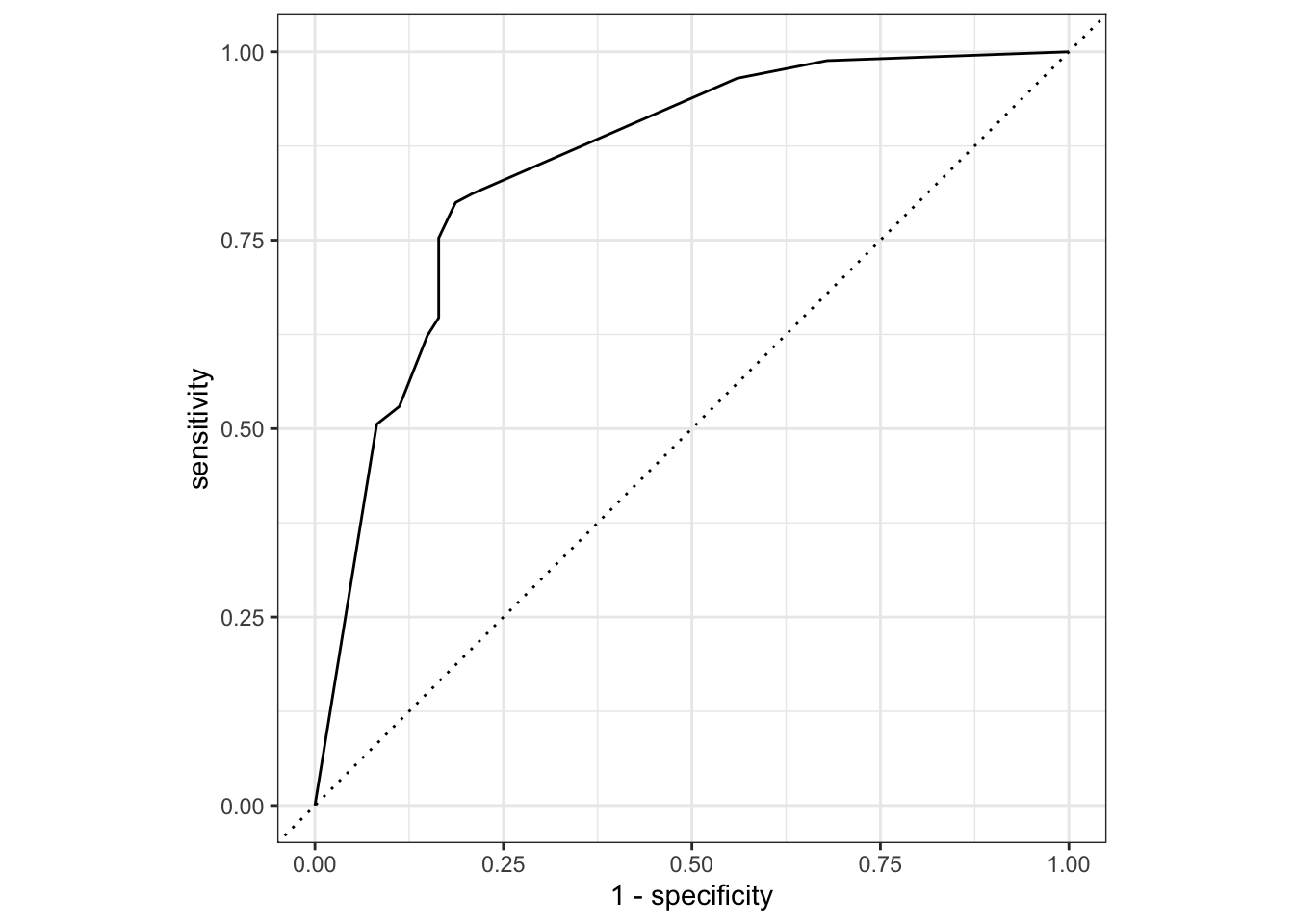
## Plot ROC curve
telecom_results %>%
  yardstick::roc_curve(truth = canceled_service, .pred_yes) %>%
  autoplot()
Comparing with the results from Assessing Model Fitting, we can find that after feature engineering, the model perform better!
Additional Note
当学完 workflow 包之后,我们在回看 recipe 包的时候,可能会存在疑问:
prep() 和 bake() 到底具有什么意义,什么时候用?这个问题tmwr书进行里说明,Max Kuhn 也讲过。一般来说,recipe object 是被直接用在 workflow 里面的,i.e.
wflow_obj <-
  workflow() %>%
  add_model(...) %>%
  add_recipe(...)
当需要debug的时候,使用prep() 和 bake()。
From Max Kuhn’s lecture notes, we learned that:
-
90% of the time, you will want to use a workflow to estimate and apply a recipe.
-
If you have an error, the original recipe object can be estimated manually with a function called
prep()(analogous tofit()). This returns the fitted recipe. This can help debug any issues. -
Another function (
bake()) is analogous topredict()and gives you the processed data back.

The tidymodels book has more details on debugging.
Machine Learning Workflows
Recall that:
-
parsnippkg is for Model Specification. -
recipepkg is for feature engineering.
We can combine models and recipes together! This is also the motivation for workflows package.
Combineing Models and Recipes
Goal: learn
workflowspackage.
The workflows package is designed for streamlining the model process. That is, combines a parsnip model and recipe object into a single workflow object.
Initialized with the workflow() function:
-
Add model object with
add_model() -
Add
recipeobject withadd_recipe()- Here must be specification, not a trained
recipe.
- Here must be specification, not a trained
Example code will use the new dataset, loans_df
loans_df <- read_rds("data/loan_df.rds")

set.seed("123")
## Create data split object
loans_split <- initial_split(
  data = loans_df,
  strata = loan_default
)

## Build training data
loans_training <- loans_split %>%
  training()

## Build test data
loans_test <- loans_split %>%
  testing()

## Check for correlated predictors
loans_training %>%
  ## Select numeric columns
  select_if(is.numeric) %>%
  ## Calculate correlation matrix
  cor()
##                 loan_amount interest_rate installment annual_income
## loan_amount     1.000000000  -0.009750748   0.9384548    0.36894798
## interest_rate  -0.009750748   1.000000000   0.0329387   -0.08849002
## installment     0.938454822   0.032938704   1.0000000    0.30850322
## annual_income   0.368947977  -0.088490024   0.3085032    1.00000000
## debt_to_income  0.138955303   0.133949453   0.1987249   -0.21357794
##                debt_to_income
## loan_amount         0.1389553
## interest_rate       0.1339495
## installment         0.1987249
## annual_income      -0.2135779
## debt_to_income      1.0000000
This time, we’ll use decision tree model,
dt_model <- decision_tree() %>%
  ## Specify the engine
  set_engine("rpart") %>%
  ## Specify the mode
  set_mode("classification")

## Build feature engineering pipeline
loans_recipe <- recipe(
  loan_default ~ .,
  data = loans_training
) %>%
  ## Correlation filter
  step_corr(all_numeric(), threshold = .85) %>%
  ## Normalize numeric predictors
  step_normalize(all_numeric()) %>%
  ## Create dummy variables
  step_dummy(all_nominal(), -all_outcomes())

loans_recipe
## Recipe
##
## Inputs:
##
##       role #variables
##    outcome          1
##  predictor          7
##
## Operations:
##
## Correlation filter on all_numeric()
## Centering and scaling for all_numeric()
## Dummy variables from all_nominal(), -all_outcomes()
workflow objects simplify the modeling process in tidymodels. With workflows, it’s possible to train a parsnip model and recipe object at the same time.
## Create a workflow
loans_dt_wkfl <- workflow() %>%
  ## Include the model object
  add_model(dt_model) %>%
  ## Include the recipe object
  add_recipe(loans_recipe)

## check
loans_dt_wkfl
## ══ Workflow ════════════════════════════════════════════════════════════════════
## Preprocessor: Recipe
## Model: decision_tree()
##
## ── Preprocessor ────────────────────────────────────────────────────────────────
## 3 Recipe Steps
##
## • step_corr()
## • step_normalize()
## • step_dummy()
##
## ── Model ───────────────────────────────────────────────────────────────────────
## Decision Tree Model Specification (classification)
##
## Computational engine: rpart
Model fitting with workflows
Training a workflow object
-
Pass workflow to
last_fit()and provide data split object -
View model evaluation results with
collect_metrics()
Behind the scenes:
-
Training and test datasets created
-
recipe trained and applied
-
Decision tree trained with training data
-
Predictions and metrics on test data
## Train the workflow
loans_dt_wkfl_fit <- loans_dt_wkfl %>%
  last_fit(split = loans_split)

## check
loans_dt_wkfl_fit
## # Resampling results
## # Manual resampling
## # A tibble: 1 × 6
##   splits            id               .metrics .notes   .predictions .workflow
##   <list>            <chr>            <list>   <list>   <list>       <list>
## 1 <split [653/219]> train/test split <tibble> <tibble> <tibble>     <workflow>
## Calculate performance metrics on test data
loans_dt_wkfl_fit %>%
  collect_metrics()
## # A tibble: 2 × 4
##   .metric  .estimator .estimate .config
##   <chr>    <chr>          <dbl> <chr>
## 1 accuracy binary         0.804 Preprocessor1_Model1
## 2 roc_auc  binary         0.857 Preprocessor1_Model1
Cross Validation
-
The
vfold_cv()function-
Trining data
-
Number of folds,
v -
Stratification variable,
strata -
Execute
set.seed()beforevfold_cv()for reporducibility -
splitsis a list column with data split objects fore creating fold
-
-
The
fit_resamplies()function-
Train a
parsnipmodel orworkflowobject -
Provide cross validation folds,
resamples -
Optional custom metric function,
metrics -
Models trained with
fit_resamples()are not able to provide predictions on new data sourcespredict()function does not accept resample objects
-
Purpose of
fit_resample()-
Explore and compare the performance profile of different model types
-
Select best performing model type and focus on model fitting efforts
-
-
Example is,
## Create cross validation folds
set.seed(1234)
loans_folds <- vfold_cv(
  loans_training,
  v = 5,
  strata = loan_default
)

## check
loans_folds
## #  5-fold cross-validation using stratification
## # A tibble: 5 × 2
##   splits            id
##   <list>            <chr>
## 1 <split [521/132]> Fold1
## 2 <split [522/131]> Fold2
## 3 <split [523/130]> Fold3
## 4 <split [523/130]> Fold4
## 5 <split [523/130]> Fold5
## Create custom metrics function
loans_metrics <- metric_set(
  yardstick::roc_auc,
  yardstick::sens,
  yardstick::spec
)

## Fit resamples
loans_dt_rs <- loans_dt_wkfl %>%
  fit_resamples(
    resamples = loans_folds,
    metrics = loans_metrics
  )

## View performance metrics
loans_dt_rs %>%
  collect_metrics()
## # A tibble: 3 × 6
##   .metric .estimator  mean     n std_err .config
##   <chr>   <chr>      <dbl> <int>   <dbl> <chr>
## 1 roc_auc binary     0.835     5 0.00982 Preprocessor1_Model1
## 2 sens    binary     0.675     5 0.0434  Preprocessor1_Model1
## 3 spec    binary     0.860     5 0.0262  Preprocessor1_Model1
Now, let’s try cross validation using logistic regression model,
logistic_model <- logistic_reg() %>%
  ## Specify the engine
  set_engine("glm") %>%
  ## Specify the mode
  set_mode("classification")

## Create workflow
loans_logistic_wkfl <- workflow() %>%
  ## Add model
  add_model(logistic_model) %>%
  ## Add recipe
  add_recipe(loans_recipe)

## Fit resamples
loans_logistic_rs <- loans_logistic_wkfl %>%
  fit_resamples(
    resamples = loans_folds,
    metrics = loans_metrics
  )

## View performance metrics
loans_logistic_rs %>%
  collect_metrics()
## # A tibble: 3 × 6
##   .metric .estimator  mean     n std_err .config
##   <chr>   <chr>      <dbl> <int>   <dbl> <chr>
## 1 roc_auc binary     0.848     5  0.0112 Preprocessor1_Model1
## 2 sens    binary     0.643     5  0.0284 Preprocessor1_Model1
## 3 spec    binary     0.863     5  0.0186 Preprocessor1_Model1
Comparing model performance profiles
The benefit of the collect_metrics() function is that it returns a tibble of cross validation results. This makes it easy to calculate custom summary statistics with the dplyr package.
## Detailed cross validation results
dt_rs_results <- loans_dt_rs %>%
  ## summarize = FALSE will provide all metric estimates for every cross validation fold
  collect_metrics(summarize = FALSE)

## Explore model performance for decision tree
dt_rs_results %>%
  group_by(.metric) %>%
  summarize(
    across(.estimate, list(
      min = min,
      median = median,
      max = max
    ), .names = "{.fn}")
  )
## # A tibble: 3 × 4
##   .metric   min median   max
##   <chr>   <dbl>  <dbl> <dbl>
## 1 roc_auc 0.812  0.826 0.867
## 2 sens    0.549  0.706 0.78
## 3 spec    0.775  0.862 0.938
## Detailed cross validation results
logistic_rs_results <- loans_logistic_rs %>%
  collect_metrics(summarize = FALSE)

## Explore model performance for logistic regression
logistic_rs_results %>%
  group_by(.metric) %>%
  summarize(
    across(.estimate, list(
      min = min,
      median = median,
      max = max
    ), .names = "{.fn}")
  )
## # A tibble: 3 × 4
##   .metric   min median   max
##   <chr>   <dbl>  <dbl> <dbl>
## 1 roc_auc 0.828  0.834 0.888
## 2 sens    0.549  0.66  0.72
## 3 spec    0.812  0.877 0.9
Hyperparamter tuning
Hyperparameters: Model parameters whose values are set prior to model training and control model complexity.
Hyperparameter tuning: Process of using cross validation to find the optimal set of hyperparameter values.
Goal: learn
tunepackage.
-
To label hyperparameters for for tuning, set them equal to
tune()inparsnipmodel specification -
Create model object with tuning parameters will let other functions know that they need to be optimized
需要调整哪个参数,就tune()哪个,在model specification 中设置:
## Set tuning hyperparameters
dt_tune_model <- decision_tree(
  cost_complexity = tune(),
  tree_depth = tune(),
  min_n = tune()
) %>%
  ## Specify engine
  set_engine("rpart") %>%
  ## Specify mode
  set_mode("classification")

## check
dt_tune_model
## Decision Tree Model Specification (classification)
##
## Main Arguments:
##   cost_complexity = tune()
##   tree_depth = tune()
##   min_n = tune()
##
## Computational engine: rpart
workflow objects can be easily updated. For example, update_model provide new decision tree model with tuning parameters.
## Create a tuning workflow
loans_tune_wkfl <- loans_dt_wkfl %>%
  ## Replace model
  update_model(dt_tune_model)

loans_tune_wkfl
## ══ Workflow ════════════════════════════════════════════════════════════════════
## Preprocessor: Recipe
## Model: decision_tree()
##
## ── Preprocessor ────────────────────────────────────────────────────────────────
## 3 Recipe Steps
##
## • step_corr()
## • step_normalize()
## • step_dummy()
##
## ── Model ───────────────────────────────────────────────────────────────────────
## Decision Tree Model Specification (classification)
##
## Main Arguments:
##   cost_complexity = tune()
##   tree_depth = tune()
##   min_n = tune()
##
## Computational engine: rpart
Random grid search
The most common method of hyperparameter tuning is grid search. This method creates a tuning grid with unique combinations of hyperparameter values and uses cross validation to evaluate their performance. The goal of hyperparameter tuning is to find the optimal combination of values for maximizing model performance.
Goal: learn
dialspackage.
-
use
parameters()to identify hyperparameters -
use
grid_random()to generate random combinations-
first arg is the results of
parameters()function -
sizearg sets the number of random combinatitions to generate
-
-
use
tune_gird()to perform hyperparameter tuning, need args:-
workfloworparsnipmodel -
resamples, cross validation object -
grid, tuning grid -
metricsfunction is Optional
-
## Hyperparameter tuning with grid search
set.seed(214)
dt_grid <- grid_random(
  parameters(dt_tune_model),
  size = 5
)

## Hyperparameter tuning
dt_tuning <- loans_tune_wkfl %>%
  tune_grid(
    ## cv resample data
    resamples = loans_folds,
    grid = dt_grid,
    metrics = loans_metrics
  )

## View results
dt_tuning %>%
  collect_metrics()
## # A tibble: 15 × 9
##    cost_complexity tree_depth min_n .metric .estimator  mean     n std_err
##              <dbl>      <int> <int> <chr>   <chr>      <dbl> <int>   <dbl>
##  1    0.0000000758         14    39 roc_auc binary     0.832     5 0.00832
##  2    0.0000000758         14    39 sens    binary     0.699     5 0.0485
##  3    0.0000000758         14    39 spec    binary     0.820     5 0.0329
##  4    0.0243                5    34 roc_auc binary     0.765     5 0.00824
##  5    0.0243                5    34 sens    binary     0.619     5 0.0195
##  6    0.0243                5    34 spec    binary     0.910     5 0.00842
##  7    0.00000443           11     8 roc_auc binary     0.808     5 0.0119
##  8    0.00000443           11     8 sens    binary     0.683     5 0.0246
##  9    0.00000443           11     8 spec    binary     0.810     5 0.0120
## 10    0.000000600           3     5 roc_auc binary     0.765     5 0.00563
## 11    0.000000600           3     5 sens    binary     0.572     5 0.0273
## 12    0.000000600           3     5 spec    binary     0.925     5 0.00692
## 13    0.00380               5    36 roc_auc binary     0.825     5 0.0109
## 14    0.00380               5    36 sens    binary     0.623     5 0.0331
## 15    0.00380               5    36 spec    binary     0.875     5 0.0228
## # … with 1 more variable: .config <chr>
## Collect detailed tuning results
dt_tuning_results <- dt_tuning %>%
  collect_metrics(summarize = FALSE)

## Explore detailed ROC AUC results for each fold
dt_tuning_results %>%
  filter(.metric == "roc_auc") %>%
  group_by(id) %>%
  summarize(
    min_roc_auc = min(.estimate),
    median_roc_auc = median(.estimate),
    max_roc_auc = max(.estimate)
  )
## # A tibble: 5 × 4
##   id    min_roc_auc median_roc_auc max_roc_auc
##   <chr>       <dbl>          <dbl>       <dbl>
## 1 Fold1       0.744          0.787       0.818
## 2 Fold2       0.748          0.802       0.819
## 3 Fold3       0.776          0.807       0.858
## 4 Fold4       0.77           0.789       0.849
## 5 Fold5       0.759          0.805       0.853
Selecting the best model
-
show_best()function displays the topnmodels based on average value ofmetric -
select_best()function will select themetricon which to evaluate performance, and returns a tibble with the best performing model and hyperparameter values -
finalize_workflow()function will finalize aworkflowthat contains a model object with tuning parameters. It will return aworkflowobject with set hyperparameter values -
last_filt()will-
Train and test datasets created
-
recipetrained and applied -
Tuned modeltrained with entire triaining dataset -
Predictions and metrics on test data
-
## Display 5 best performing models
dt_tuning %>%
  show_best(metric = "roc_auc", n = 5)
## # A tibble: 5 × 9
##   cost_complexity tree_depth min_n .metric .estimator  mean     n std_err
##             <dbl>      <int> <int> <chr>   <chr>      <dbl> <int>   <dbl>
## 1    0.0000000758         14    39 roc_auc binary     0.832     5 0.00832
## 2    0.00380               5    36 roc_auc binary     0.825     5 0.0109
## 3    0.00000443           11     8 roc_auc binary     0.808     5 0.0119
## 4    0.0243                5    34 roc_auc binary     0.765     5 0.00824
## 5    0.000000600           3     5 roc_auc binary     0.765     5 0.00563
## # … with 1 more variable: .config <chr>
## Select based on best performance
best_dt_model <- dt_tuning %>%
  ## Choose the best model based on roc_auc
  select_best(metric = "roc_auc")

## check
best_dt_model
## # A tibble: 1 × 4
##   cost_complexity tree_depth min_n .config
##             <dbl>      <int> <int> <chr>
## 1    0.0000000758         14    39 Preprocessor1_Model1
## Finalize your workflow
final_loans_wkfl <- loans_tune_wkfl %>%
  finalize_workflow(best_dt_model)

final_loans_wkfl
## ══ Workflow ════════════════════════════════════════════════════════════════════
## Preprocessor: Recipe
## Model: decision_tree()
##
## ── Preprocessor ────────────────────────────────────────────────────────────────
## 3 Recipe Steps
##
## • step_corr()
## • step_normalize()
## • step_dummy()
##
## ── Model ───────────────────────────────────────────────────────────────────────
## Decision Tree Model Specification (classification)
##
## Main Arguments:
##   cost_complexity = 7.58290839567418e-08
##   tree_depth = 14
##   min_n = 39
##
## Computational engine: rpart
## Train finalized decision tree workflow
loans_final_fit <- final_loans_wkfl %>%
  last_fit(split = loans_split)

## View performance metrics
loans_final_fit %>%
  collect_metrics()
## # A tibble: 2 × 4
##   .metric  .estimator .estimate .config
##   <chr>    <chr>          <dbl> <chr>
## 1 accuracy binary         0.763 Preprocessor1_Model1
## 2 roc_auc  binary         0.850 Preprocessor1_Model1
## Create an ROC curve
loans_final_fit %>%
  ## Collect predictions
  collect_predictions() %>%
  ## Calculate ROC curve metrics
  roc_curve(truth = loan_default, .pred_yes) %>%
  ## Plot the ROC curve
  autoplot()
Reference
-
Tidy Modeling with R books free online.
- Tidy Modeling with R Book Club,这个是tidy modeling with r 书的辅导材料,加入了总结,很不错
-
ISLR tidymodels Labs code example using tidymodels.
-
An Introduction to Statistical Learning 2nd version newest book