Orthogonal vs Non-orthogonal Learning

Setting

We compare the performance of the naive and orthogonal methods in a computational experiment where $p=n=100$, ${\beta }_j=1/j^2$, $({\gamma }_{DW}{)}_j=1/j^2$ and $$Y=1\cdot D+{\beta }^{\prime }W+{ϵ}_Y$$

where $W\sim N(0,I)$, ${ϵ}_Y\sim N(0,1)$, and $$D={\gamma }_{DW}^{\prime }W+\tilde{D}$$ where $\tilde{D}\sim N(0,1)/4$.

Note that: $\tilde{D}$ is the residual from the projection $D\sim W$.

• The true treatment effect here is 1.

• From the plots produced in this post (estimate minus ground truth), we show that the naive single-selection estimator is heavily biased (lack of Neyman orthogonality in its estimation strategy), while the orthogonal estimator based on partialling out, is approximately unbiased and Gaussian.

Simulation

library(hdm)
library(ggplot2)

# Initialize constants
B <- 10000  # Number of iterations
n <- 100  # Sample size
p <- 100  # Number of features

# Initialize arrays to store results
Naive <- rep(0, B)
Orthogonal <- rep(0, B)


lambdaYs <- rep(0, B)
lambdaDs <- rep(0, B)

for (i in 1:B) {
  # Generate parameters
  beta <- 1 / (1:p)^2
  gamma <- 1 / (1:p)^2

  # Generate covariates / random data
  X <- matrix(rnorm(n * p), n, p)
  D <- X %*% gamma + rnorm(n) / 4

  # Generate Y using DGP
  Y <- D + X %*% beta + rnorm(n)

  # Single selection method
  rlasso_result <- hdm::rlasso(Y ~ D + X)  # Fit lasso regression
  sx_ids <- which(rlasso_result$coef[-c(1, 2)] != 0)  # Selected covariates

  # Check if any Xs are selected
  if (sum(sx_ids) == 0) {
    Naive[i] <- lm(Y ~ D)$coef[2]  # Fit linear regression with only D if no Xs are selected
  } else {
    Naive[i] <- lm(Y ~ D + X[, sx_ids])$coef[2]  # Fit linear regression with selected X otherwise
  }

  # Partialling out / Double Lasso

  fitY <- hdm::rlasso(Y ~ X, post = TRUE)
  resY <- fitY$res

  fitD <- hdm::rlasso(D ~ X, post = TRUE)
  resD <- fitD$res

  Orthogonal[i] <- lm(resY ~ resD)$coef[2]  # Fit linear regression for residuals
}

Making a Nice Plot

# Specify ratio
img_width <- 15
img_height <- img_width / 2

# Create a data frame for the estimates
df <- data.frame(
  Method = rep(c("Naive", "Orthogonal"), each = B),
  Value = c(Naive - 1, Orthogonal - 1)
)

# Create the histogram using ggplot2
hist_plot <- ggplot(df, aes(x = Value, fill = Method)) +
  geom_histogram(binwidth = 0.1, color = "black", alpha = 0.7) +
  facet_wrap(~Method, scales = "fixed") +
  labs(
    title = "Distribution of Estimates (Centered around Ground Truth)",
    x = "Bias",
    y = "Frequency"
  ) +
  geom_vline(xintercept = 0, color = "red", linetype = "dashed") +
  scale_x_continuous(breaks = seq(-2, 1.5, 0.5)) +
  theme_minimal() +
  theme(
    plot.title = element_text(hjust = 0.5),  # Center the plot title
    strip.text = element_text(size = 10),  # Increase text size in facet labels
    legend.position = "none", # Remove the legend
    panel.grid.major = element_blank(),  # Make major grid lines invisible
    # panel.grid.minor = element_blank(),  # Make minor grid lines invisible
    strip.background = element_blank()  # Make the strip background transparent
  ) +
  theme(panel.spacing = unit(2, "lines"))  # Adjust the ratio to separate subplots wider

# Set a wider plot size
options(repr.plot.width = img_width, repr.plot.height = img_height)

# Display the histogram
print(hist_plot)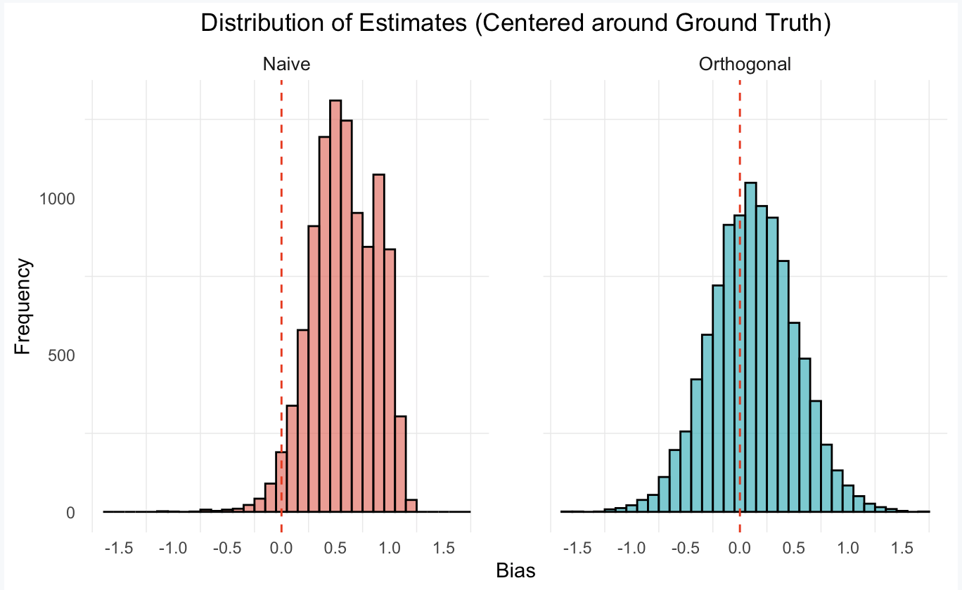

Conclusion: As we can see from the above bias plots (estimates minus the ground truth effect of 1), the double lasso procedure concentrates around zero whereas the naive estimator does not.

Reference

CausalAIBook Notebook