1.1 Model probabilites

The short story is that the Beta distribution can be understood as representing a distribution of probabilities, that is, it represents all the possible values of a probability when we don’t know what that probability is.

1.2 Generalization of uniform

Give me a continuous and bounded random variable, em, except the Uniform distribution. That is another way to look at beta distribution, continuous and bounded between 0, 1; also the density is not flat. $$X\sim Beta(a,b),\text{ where }a>0,b>0.$$

$$f_X(x)=c\cdot x^{a-1}(1-x{)}^{b-1},\text{ where }x>0.$$

What is $c$? Just a normalization constant. We’ll get the value of $c$ later.

2.1 Bank and Post Office Story

Let $X$ be the waiting time at Bank,

$$X\sim Gamma(n_1,\lambda )$$

Let $Y$ be the waiting time at Post Office,

$$Y\sim Gamma(n_2,\lambda )$$

Assume $X$ and $Y$ are independent.

Then, what is the distribution of the proportion $\frac{X}{X+Y}$?

Define $T=X+Y$ be the total waiting time.

Clearly, $T\sim Gamma(n_1+n_2,\lambda )$, proved by MGF.

Define $W=\frac{X}{X+Y}$ , the proportion of waiting time at Bank to the total waiting time.

What is the distribution of $W$?

We need to derive $f_W(w)$, but first let’s find the joint pdf $f_{T,W}(t,w)$ $$\begin{array}{rl}{f}_{T,W}(t,w)& =f_{X,Y}(x,y)\left|\frac{\partial (x,y)}{\partial (t,w)}\right|\\ & =\frac{1}{\mathrm{\Gamma }(n_1)}{\lambda }^{n_1}{x}^{n_1-1}{e}^{-\lambda x}\frac{1}{\mathrm{\Gamma }(n_2)}{\lambda }^{n_2}{x}^{n_2-1}{e}^{-\lambda y}|-t|\\ & ={\lambda }^{n_1+n_2}{t}^{n_1+n_2-1}{e}^{\lambda t}\frac{1}{\mathrm{\Gamma }(n_1)\mathrm{\Gamma }(n_2)}{w}^{n_1-1}(1-w{)}^{n_2-1}\\ & =\frac{{\lambda }^{n_1+n_2}{t}^{n_1+n_2-1}{e}^{\lambda t}}{\mathrm{\Gamma }(n_1+n_2)}\frac{\mathrm{\Gamma }(n_1+n_2)}{\mathrm{\Gamma }(n_1)\mathrm{\Gamma }(n_2)}{w}^{n_1-1}(1-w{)}^{n_2-1}\\ & =f_T(t)\frac{\mathrm{\Gamma }(n_1+n_2)}{\mathrm{\Gamma }(n_1)\mathrm{\Gamma }(n_2)}{w}^{n_1-1}(1-w{)}^{n_2-1}\end{array}$$

Then we find the marginal,

Since $f_W(w)$ is the pdf needed to be integrated to 1,

$${\int }_0^1\frac{\mathrm{\Gamma }(n_1+n_2)}{\mathrm{\Gamma }(n_1)\mathrm{\Gamma }(n_2)}{w}^{n_1-1}(1-w{)}^{n_2-1}dw\equiv 1$$

so the normalization constant should be

$$c=\frac{\mathrm{\Gamma }(n_1+n_2)}{\mathrm{\Gamma }(n_1)\mathrm{\Gamma }(n_2)}:=\frac{1}{B(n_1,n_2)}$$

2.2 plots

library(zetaEDA)
library(ggfortify)
enable_zeta_ggplot_theme()

Let’s check Beta density for some different parameters value.

How about $a=b=1$? The Beta(1,1) is just the Unif(0,1).

ggdistribution(func = dbeta, x = seq(0, 1, .01), shape1 = 1, shape2 = 1) +
  labs(title = "Beta Density with a = 1, b = 1")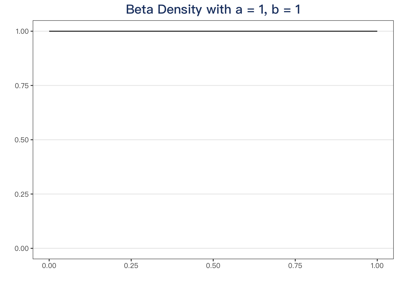

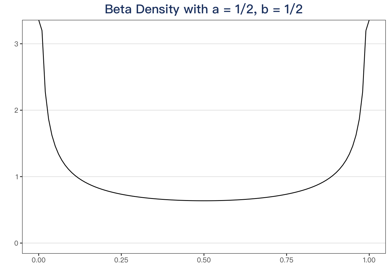
How about $a=b=\frac{1}{2}$?

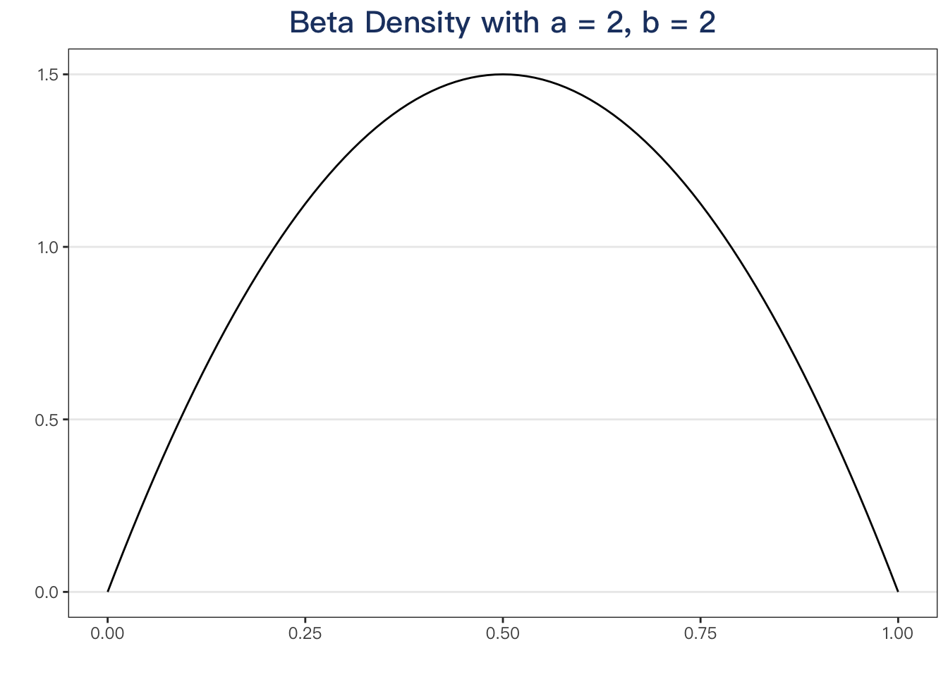
How about $a=b=2$?

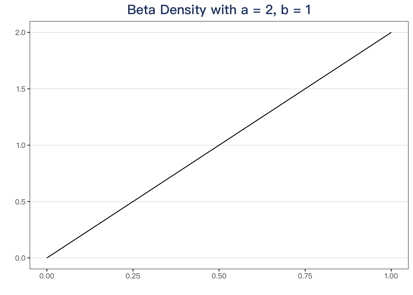
How about $a=2,b=1$?

One more,

p <- ggdistribution(func = dbeta, x = seq(0, 1, .01), shape1 = 1.5, shape2 = 5, colour = "tomato", linetype = "dashed")

ggdistribution(func = dbeta, x = seq(0, 1, .01), shape1 = 5, shape2 = 1.5, colour = "blue", p = p) +
  labs(title = "Red: a = 1.5, b = 5\n Blue: a = 5, b = 1.5")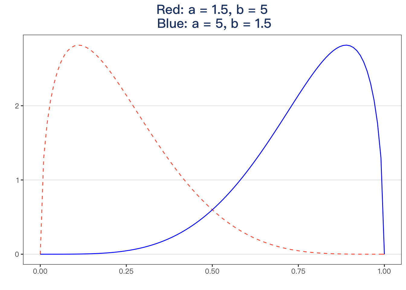

For more checking, click this link and try some parameters to check the density curve.

Have fun!