Beta Distribution — Intuition, Derivation, and Examples
Motivation
Model probabilities
The Beta distribution is a probability distribution on probabilities.
The Beta distribution can be understood as representing a distribution of probabilities, that is, it represents all the possible values of a probability when we don’t know what that probability is. For example,
-
the Click-Through Rate of your advertisement
-
the conversion rate of customers actually purchasing in your store
-
how likely the customer will become “inactive”
Because the Beta distribution models a probability, its domain is bounded between 0 and 1.
Generalization of Uniform Distribution
Give me a continuous and bounded random variable except the Uniform Distribution. This is another way to look at beta distribution, continuous and bounded between 0 and 1; also the density is not flat.
$$ X \sim Beta(a, b), \text{ where } a>0, \ b>0. $$ $$ f_X(x) = c \cdot x ^{a-1}(1-x)^{b-1}, \text{ where } x>0. $$What is $c$ ? Just a normalization constant! We’ll find the value of $c$ later.
Conjugate Prior
The Beta distribution is the conjugate prior for the Bernoulli, binomial, negative binomial and geometric distributions (seems like those are the distributions that involve success & failure) in Bayesian inference.
Computing a posterior using a conjugate prior is very convenient, because you can avoid expensive numerical computation involved in Bayesian Inference.Conjugate prior = Convenient prior
For example, the beta distribution is a conjugate prior to the binomial. If we choose to use the beta distribution Beta(α, β) as a prior, during the modeling phase, we already know the posterior will also be a beta distribution. Therefore, after carrying out more experiments, you can compute the posterior simply by adding the number of successes (x), and failures (n-x) to the existing parameters α, β respectively, instead of multiplying the likelihood with the prior distribution. The posterior also becomes a Beta distribution with parameters (x+α, n-x+β).
What is the Intuition?
The intuition for the beta distribution comes into play when we look at it from the lens of the binomial distribution.
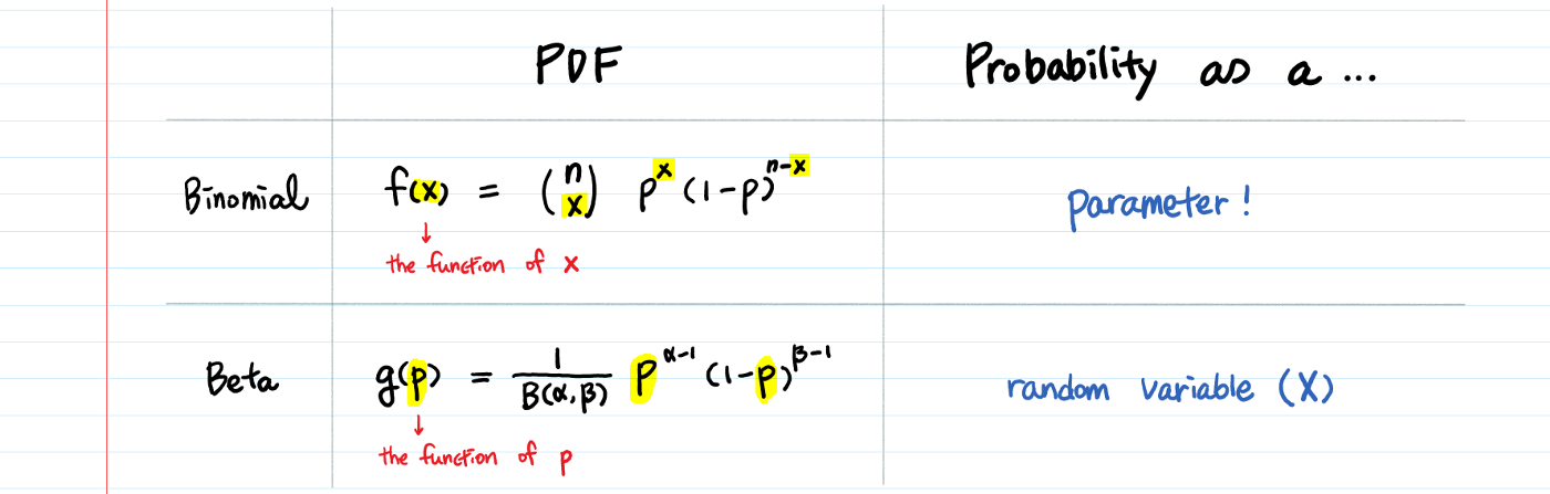
The difference between the binomial and the beta is that the former models the number of successes (x), while the latter models the probability (p) of success.
In other words, the probability is a parameter in binomial; In the Beta, the probability is a random variable.
Interpretation of α, β
You can think of α-1 as the number of successes and β-1 as the number of failures, just like n & n-x terms in binomial.
You can choose the α and β parameters however you think they are supposed to be.
- If you think the probability of success is very high, let’s say 90%, set 90 for α and 10 for β.
- If you think otherwise, 90 for β and 10 for α.
As α becomes larger (more successful events), the bulk of the probability distribution will shift towards the right, whereas an increase in β moves the distribution towards the left (more failures).
Also, the distribution will narrow if both α and β increase, for we are more certain.
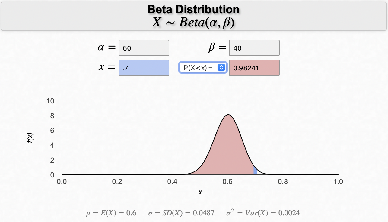
Dr. Bognar at the University of Iowa built the calculator for Beta distribution, which I found useful and beautiful. You can experiment with different values of α and β and visualize how the shape changes.
Derivation
In this section, we’ll derive Beta distribution using the Beta-Gamma Connections.
Fraction of Waiting Time
Let $X$ be the waiting time at Bank,
$$ X \sim Gamma(n_1, \lambda) $$Let $Y$ be the waiting time at Post Office,
$$ Y \sim Gamma(n_2, \lambda) $$Assume $X$ and $Y$ are independent. What is the distribution of the proportion $\frac{X}{X+Y}$ ?
Solution:
Let $T := X+Y$ be the total waiting time. Clearly, $T \sim Gamma(n_1+n_2, \lambda)$, you can prove it by MGF.
Let $W =: \frac{X}{X+Y}$ be the proportion of waiting time at Bank to the total waiting time. We need to find the PDF of $W$.
The idea is to find the joint PDF $f_{T,W}(t,w)$ at first, and then get the marginal distribution.
$$ \begin{aligned}f_{T,W}(t,w) &= f_{X,Y}(x,y) \left | \frac{\partial(x,y)}{\partial(t,w)} \right|\\ &= \frac{1}{\Gamma(n_1)}\lambda^{n_1}x^{n_1 - 1}e^{-\lambda x} \frac{1}{\Gamma(n_2)}\lambda^{n_2}x^{n_2 - 1}e^{-\lambda y} \left|-t\right|\\ &= \lambda^{n_1+n_2}t^{n_1+n_2-1}e^{-\lambda t} \frac{1}{\Gamma(n_1)\Gamma(n_2)}w^{n_1 - 1}(1-w)^{n_2-1}\\ &= \frac{\lambda^{n_1+n_2}t^{n_1+n_2-1}e^{-\lambda t}}{\Gamma(n_1+n_2)} \frac{\Gamma(n_1+n_2)}{\Gamma(n_1)\Gamma(n_2)}w^{n_1 - 1}(1-w)^{n_2-1}\\ &= f_T(t) \frac{\Gamma(n_1+n_2)}{\Gamma(n_1)\Gamma(n_2)}w^{n_1 - 1}(1-w)^{n_2-1}\end{aligned} $$Integrating $t$ out to get the marginal:
$$ \begin{aligned}f_W(w) &= \int_0^\infty f_{T,W}(t,w) dt \\&= \frac{\Gamma(n_1+n_2)}{\Gamma(n_1)\Gamma(n_2)}w^{n_1 - 1}(1-w)^{n_2-1} \cdot\int_0^\infty f_T(t)dt \\&= \frac{\Gamma(n_1+n_2)}{\Gamma(n_1)\Gamma(n_2)}w^{n_1 - 1}(1-w)^{n_2-1} \end{aligned} $$Here we have Beta,
$$W \sim Beta(n_1, n_2)$$ REMARK: the above result also proves W and T and independent!Beta Function as a normalizing constant
Note that, $f_W(w)$ is a PDF needed to be integrated to 1,
$$ \int_0^1\frac{\Gamma(n_1+n_2)}{\Gamma(n_1)\Gamma(n_2)}w^{n_1 - 1}(1-w)^{n_2-1} dw \equiv 1 $$So the normalization constant should be,
$$ c = \frac{\Gamma(n_1+n_2)}{\Gamma(n_1)\Gamma(n_2)} := \frac{1}{B(n_1, n_2)} $$Mean of Beta distribution
As a byproduct in the above derivation, we get that fact that W and T are independent. Then, we can use this to derive the mean of Beta distribution,
$$E(WT) = E(W)E(T) \implies E(X) =E\left(\frac{X}{X+Y}\right)E(X+Y),$$rearrange to get,
$$E\left(\frac{X}{X+Y}\right) = \frac{E(X)}{E(X+Y)}$$This result is clear Not True in general, but under our setting, we have this interesting result.
We can use this result to find the mean of $W \sim Beta(a, b)$ without the slightest trace of calculus.
$$E(W)=E\left(\frac{X}{X+Y}\right)=\frac{E(X)}{E(X+Y)}=\frac{a / \lambda}{a / \lambda+b / \lambda}=\frac{a}{a+b}$$Getting Beta parameters in practice
The Beta distribution is the conjugate prior for many common distributions. We use it a lot. But in practice, how to figure out its parameters? It is sometimes useful to estimate quickly the parameters of the Beta distribution using the method of moments:
$$X \sim Beta(\alpha, \beta),$$ $$\alpha + \beta = \frac{E(X)(1-E(X))}{Var(X)} - 1,$$ $$\alpha = (\alpha + \beta)E(X),$$ $$\beta = (\alpha + \beta)(1 - E(X))$$Here is the R code:
# calculate beta params using method of moments
cal_beta_params <- function(meanX, sdX) {
  varX <- sdX^2
  sum_ab <- meanX * (1 - meanX) / varX - 1
  a <- sum_ab * meanX
  b <- sum_ab * (1 - meanX)
  # return
  c("shape" = a, "scale" = b)
}

# example
cal_beta_params(meanX = 0.136, sdX = 0.103)
##    shape    scale
## 1.370320 8.705559
Summary
To summarize, the bank–post office story tells us that: when we add independent Gamma r.v.s $X$ and $Y$ with the same rate $\lambda$ ,
-
the total $X+Y$ has a Gamma distribution;
-
the fraction $\frac{X}{X+Y}$ has a Beta distribution;
-
the total is independent of the fraction.
Examples
The PDF of Beta distribution can be U-shaped with asymptotic ends, bell-shaped, strictly increasing/decreasing or even straight lines. As you change α or β, the shape of the distribution changes.
I. Bell-Shape
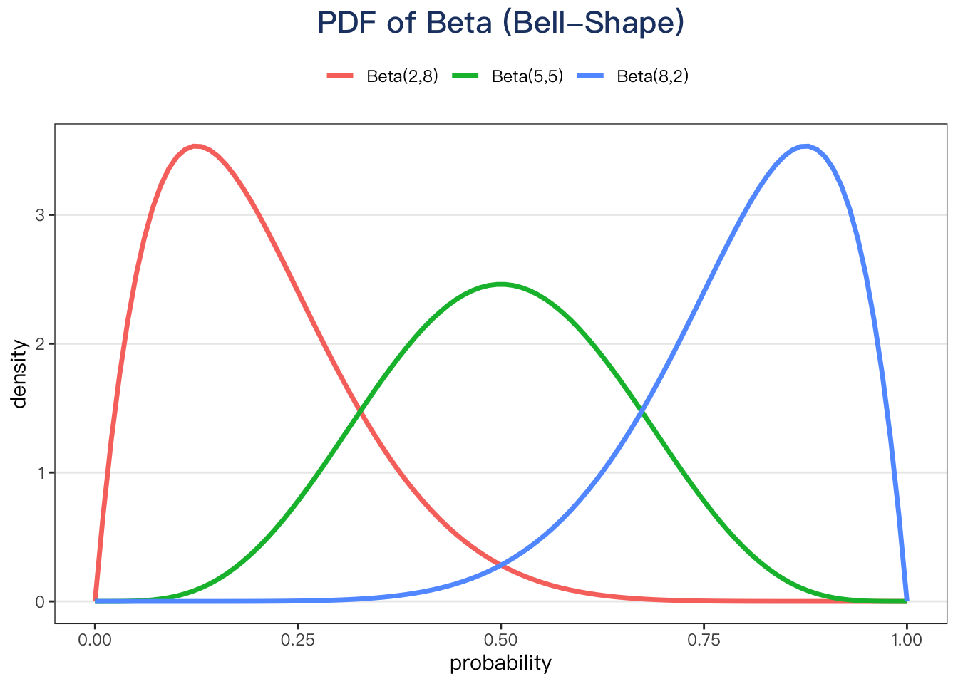
The PDF of a beta distribution is approximately normal if α + β is large enough and α & β are approximately equal.
Intuition behind Bell-Shape
Why would Beta(2,2) be bell-shaped?
If you think:
-
α-1 as the number of successes
-
β-1 as the number of failures
-
Beta(2,2) means you got 1 success and 1 failure
So it makes sense that the probability of the success is highest at 0.5.
Also, Beta(1,1) would mean you got zero for the head and zero for the tail. Then, your guess about the probability of success should be the same throughout [0,1]. The horizontal straight line confirms it.
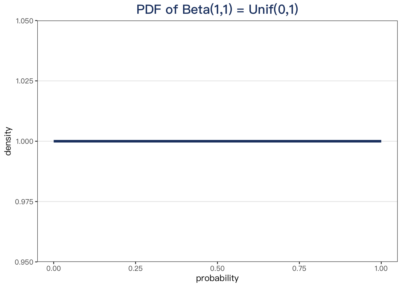
II. Straight Lines
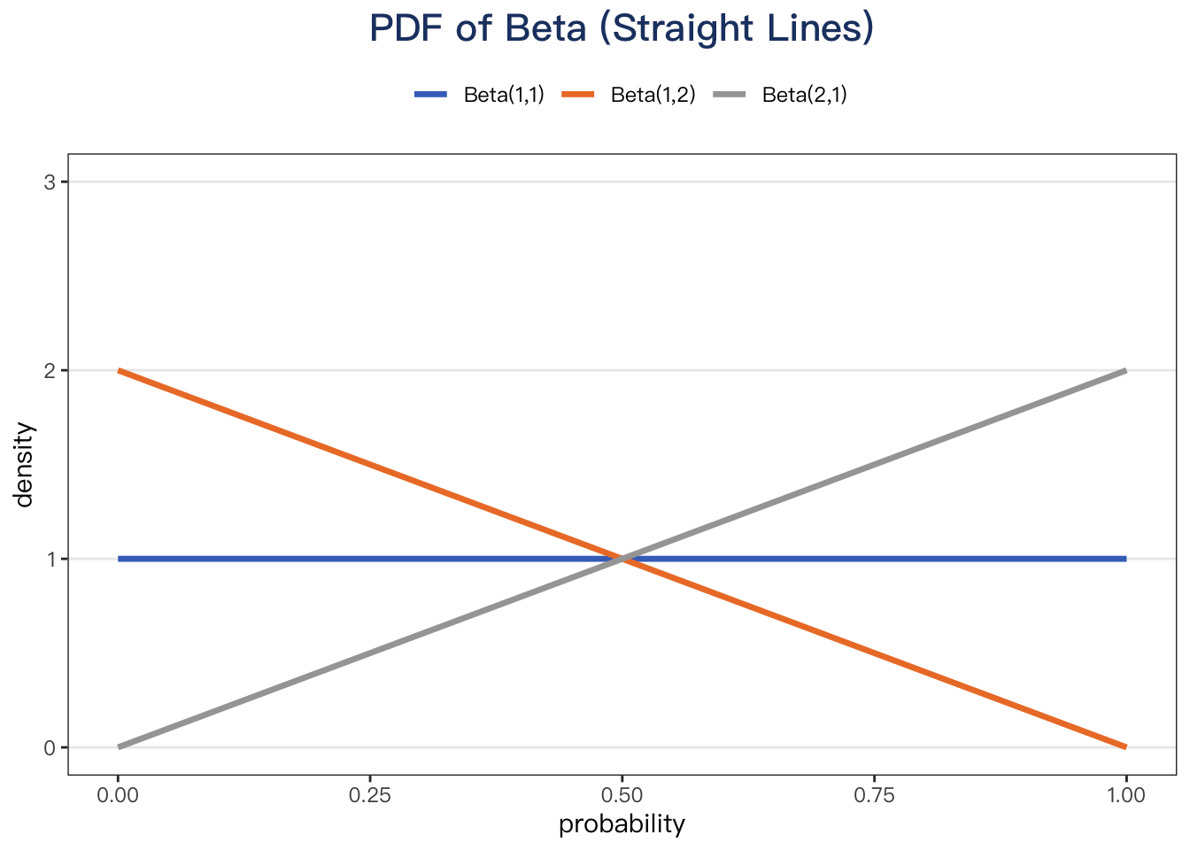
α = 1 or β = 1, the beta PDF can be a straight line.
III. U-Shape
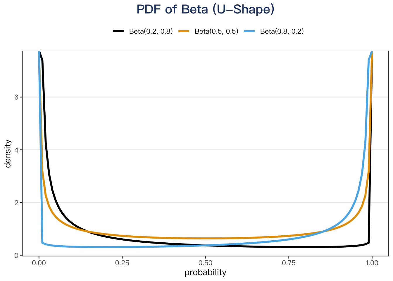 When $\alpha < 1, \beta<1$ the PDF of the Beta is U-shaped.