Beta distribution as a prior

Introduction

The Beta distribution is a useful probability distribution when you want model uncertainty over a parameter bounded between 0 and 1.

In this post, we’ll explore how the two parameters of the Beta distribution determine its shape.

One way to see how the shape parameters of the Beta distribution affect its shape is to generate a large number of random draws using the rbeta(n, shape1, shape2) function and visualize these as a histogram.

Beta(1,1)

# Explore using the rbeta function
beta_sample <- rbeta(n = 1000000, shape1 = 1, shape2 = 1)

# Visualize the results
hist(beta_sample)

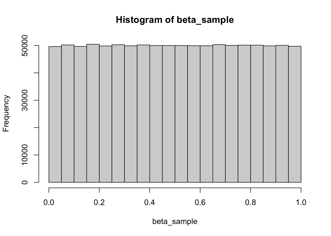
A Beta(1,1) distribution is the same as a uniform distribution between 0 and 1. It is useful as a so-called non-informative prior as it expresses than any value from 0 to 1 is equally likely.

Discover shape parameters

What happened if you set shape parameters to negative numbers?

# Modify the parameters
beta_sample <- rbeta(n = 1000000, shape1 = -1, shape2 = 1)

# Explore the results
head(beta_sample)

## [1] NaN NaN NaN NaN NaN NaN

Yes, NaN stands for not a number and the reason you got a lot of NaNs is that the Beta distribution is only defined when its shape parameters are positive.

# Modify the parameters
beta_sample <- rbeta(n = 1000000, shape1 = 100, shape2 = 100)

# Visualize the results
hist(beta_sample)

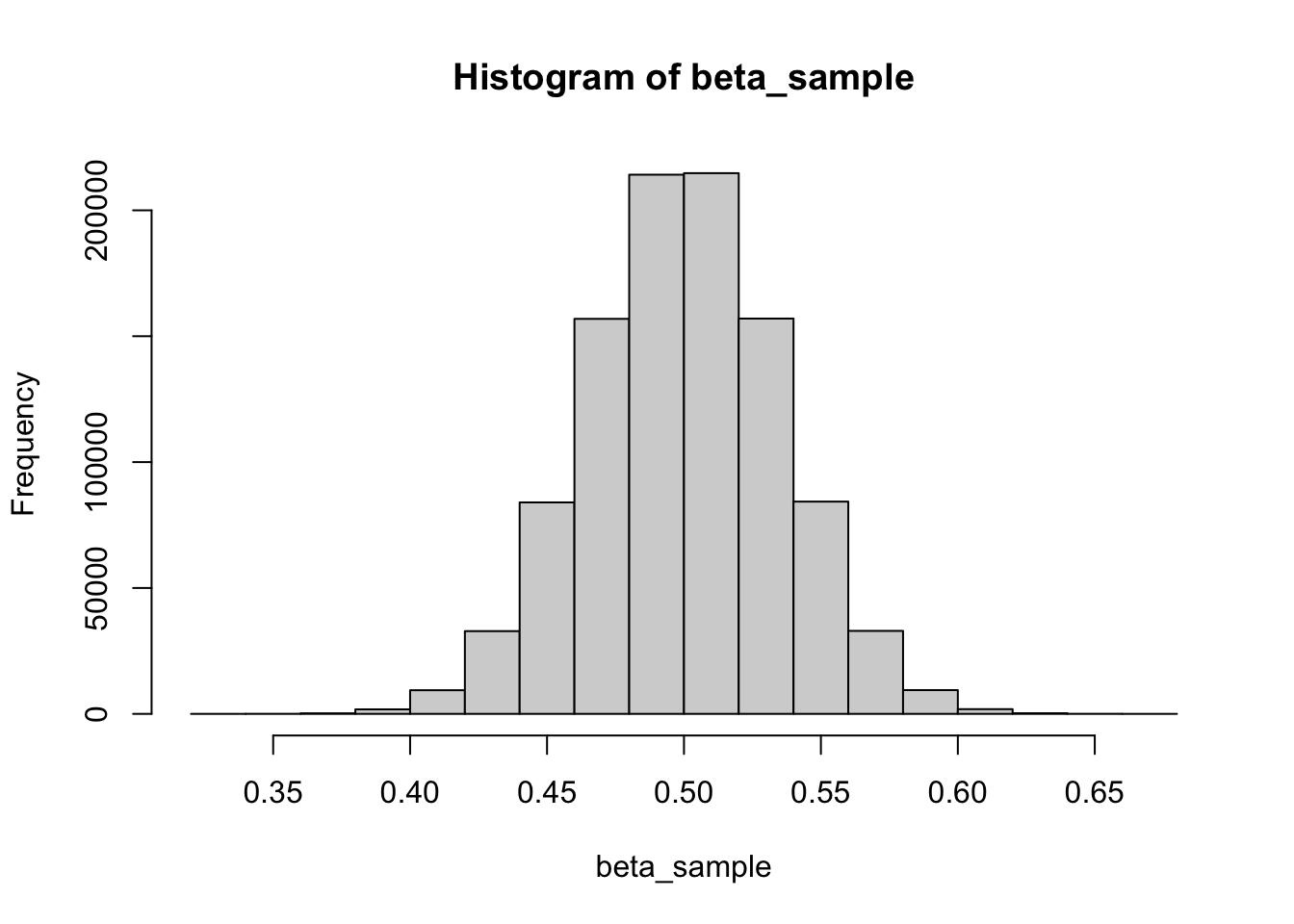
So the larger the shape parameters are, the more concentrated the beta distribution becomes. When used as a prior, this Beta distribution encodes the information that the parameter is most likely close to 0.5 .

# Modify the parameters
beta_sample <- rbeta(n = 1000000, shape1 = 100, shape2 = 20)

# Visualize the results
hist(beta_sample)

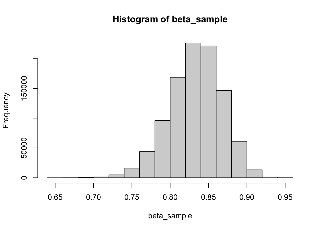
So the larger the shape1 parameter is the closer the resulting distribution is to 1.0 and the larger the shape2 the closer it is to 0.