1.1 Some notation

For an customer,

Define:

\[ x = \text{the number of purchase,} \]

\[ t_i = \text{the time of ith purchase}, \ \text{ where } 1 \le t_i \le t_x, \]

\[ t_x = \text{the time of last purchase in the history,} \]

\[ T = \text{total time being observed} \]

Next, we’ll show that it is sufficient to use individual’s \((x, t_x, T)\) to describe his/her purchase behavior in Pareto/NBD model.

1.2 Conditional on \(\lambda\) and \(\mu\)

Assume a customer’s \(x\) transactions occurred during the period \((0,T]\); we denote these times by \(t_1, t_2, t_3, \cdots, t_x\).

There are two possible ways this pattern of transactions could arise:

1. The customer is still alive at the end of the observation period (i.e., \(\tau > T\) ), the individual-level likelihood function is simply the product of the (inter-transaction-time) exponential pdf and the associated survivor function:

2. The customer became inactive at some time \(\tau\) in the interval \((t_x, T]\) (i.e. \(\tau \in (t_x, T]\)), in which case the individual-level likelihood function is

Note that in both cases, information on when each of the x transactions occurred is not required.

We can replace \(t_1, ...t_x\) , \(T\) with \((x, t_x , T)\) where, by definition, \(t_x = 0\) when \(x = 0\). In other words, \(t_x\), \(x\) and \(T\) are sufficient summaries of a customer’s transaction history. Using direct marketing terminology, \(t_x\) is recency and \(x\) is frequency.

由以上两个事实可知，无需知晓客户每次的购买时间，第一次消费时间、最后一次消费时间、消费频次 作为充分统计量，已经足够我们导出似然函数了！

Removing the conditioning on \(\tau\) gives us the following expression for the individual-level likelihood function:

1.3 Removing the Conditioning on \(\lambda\) and \(\mu\)

We remove the conditioning on \(\lambda\) and \(\mu\) by taking the expectation of \(L(\lambda, \mu | x, t_x , T)\) over the distributions of \(\lambda\) and \(\mu\) :

\[ L\left(r, \alpha, s, \beta \mid x, t_{x}, T\right)=\int_{0}^{\infty} \int_{0}^{\infty} L\left(\lambda, \mu \mid x, t_{x}, T\right) g(\lambda \mid r, \alpha) g(\mu \mid s, \beta) d \lambda d \mu \]

The computation is tedious, check the paper “A Note on Deriving the Pareto/NBD Model and Related Expressions” to know the details.

1.4 MLE for \(r, \alpha, s, \beta\)

Since we have derived the likelihood function \(L\left(r, \alpha, s, \beta \mid x, t_{x}, T\right)\), the 4 Pareto/NBD model parameters \((r, \alpha, s, \beta)\) can be estimated via the method of MLE. Specifically, suppose we have a sample of \(N\) customers, where customer \(i\) had \(x_i\) transactions in the period \((0, T_i ]\), with the last transaction occurring at \(t_{x_i}\) . The sample log-likelihood function is given by

\[ L L(r, \alpha, s, \beta)=\sum_{i=1}^{N} \ln \left[L\left(r, \alpha, s, \beta \mid x_{i}, t_{x_{i}}, T_{i}\right)\right]. \]

This can be maximized using standard numerical optimization routines. Therefore, we will obtain 4 maximum likelihood estimators \((\widehat{r} \ , \ \widehat{\alpha} \ , \ \widehat{s} \ , \ \widehat{\beta})\)

2.1 Mean of the Pareto/NBD Model

Given that the number of transactions follows a Poisson process while the customer is alive,

1. if \(\tau > t\), the expected number of transactions is simply \(\lambda t\).
2. if \(\tau \le t\), the expected number of transactions in the interval (0, τ] is \(\lambda \tau\).

Removing the conditioning on the time at which the customer becomes inactive, it follows that the expected number of transactions in the time interval \((0, t]\), conditional on \(\lambda\) and \(\mu\), is

\[ \begin{aligned} E[X(t) \mid \lambda, \mu] &=\lambda t P(\tau>t \mid \mu)+\int_{0}^{t} \lambda \tau f(\tau \mid \mu) d \tau \\ &=\lambda t e^{-\mu t}+\lambda \int_{0}^{t} \mu \tau e^{-\mu \tau} d \tau \\ &=\lambda t e^{-\mu t}+\frac{\lambda}{\mu} \int_{0}^{t} \mu^{2} \tau e^{-\mu \tau} d \tau, \text{where integrand is an Erlang-2} \\ &=\lambda t e^{-\mu t}+\frac{\lambda}{\mu}\left\{1-e^{-\mu t}-\mu t e^{-\mu t}\right\} \\ &=\frac{\lambda}{\mu}-\frac{\lambda}{\mu} e^{-\mu t} \end{aligned} \]

Now removing the Conditioning on \(\lambda\) and \(\mu\),

2.2 Derivation of PAlive

The probability that a customer with purchase history \((x, t_x , T)\) is “alive” at time \(T\) is \(P(\tau > T)\).

As the \(\lambda\) and \(\mu\) are unobserved, we compute \(P(alive | x, t_x , T)\) for a randomly-chosen individual by taking the expectation of the above result over the distribution of \(\lambda\) and \(\mu\) , updated to take account of the information \((x, t_x , T)\):

By Bayes’ theorem, the joint posterior distribution of \(\lambda\) and \(\mu\) is

\[ g\left(\lambda, \mu \mid r, \alpha, s, \beta, x, t_{x}, T\right)=\frac{L\left(\lambda, \mu \mid x, t_{x}, T\right) g(\lambda \mid r, \alpha) g(\mu \mid s, \beta)}{L\left(r, \alpha, s, \beta \mid x, t_{x}, T\right)} \]

Thus,

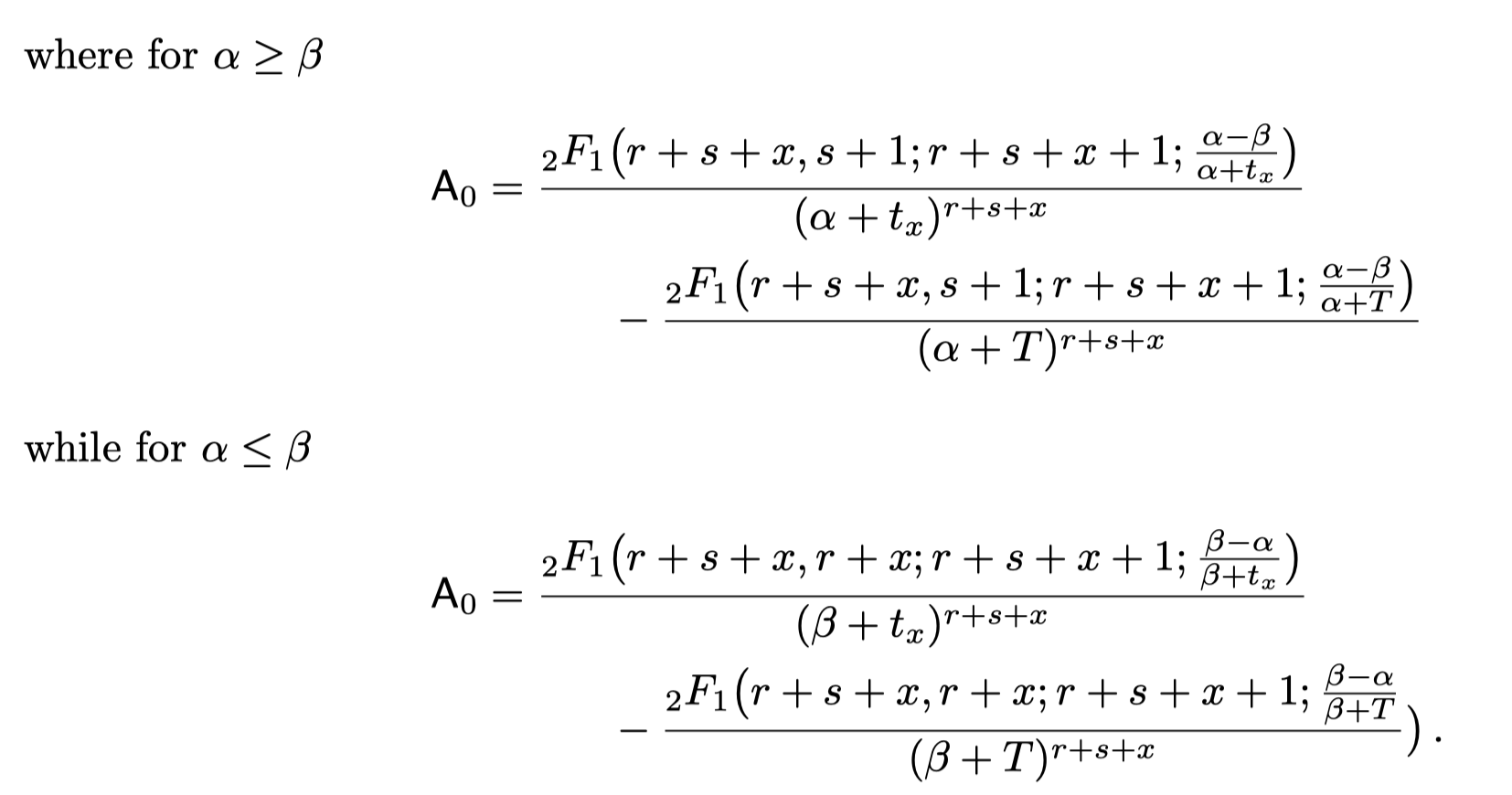
For details check the reference paper. Note that, the above result is the formula to calculate PAlive used in BTYD 📦 implemented in R.

2.3 Conditional Expectation of Transactions

Let random variable \(Y(t) = \text{num of purchase made in } (T, T+t]\). We are interested in computing \(E(Y(t)|x, t_x, T)\), the expected number of purchase in the period \((T, T+t]\) for a customer with purchase history \((x, t_x, T)\).

If the customer is active at \(T\),

\[ \begin{array}{l} &E[Y(t) \mid \lambda, \mu, \text { alive at } T]\\ &=\lambda t P(\tau>T+t \mid \mu, \tau>T)+\int_{T}^{T+t} \lambda \tau f(\tau \mid \mu, \tau>T) d \tau\\ &=\lambda t e^{-\mu t}+\lambda \int_{0}^{t} \mu \tau e^{-\mu \tau} d \tau \\ &=\frac{\lambda}{\mu}-\frac{\lambda}{\mu} e^{-\mu t} \end{array} \]

Of course we don’t know whether a customer is alive at \(T\); therefore

\[ E\left[Y(t) \mid \lambda, \mu, x, t_{x}, T\right]=E[Y(t) \mid \lambda, \mu, \text { alive at } T] P\left(\tau>T \mid \lambda, \mu, x, t_{x}, T\right) \]

Also, since \(\lambda\) and \(\mu\) are unobserved, we need to integrate them out:

\[ \begin{array}{c} E\left[Y(t) \mid r, \alpha, s, \beta, x, t_{x}, T\right]=\int_{0}^{\infty} \int_{0}^{\infty}\left\{E[Y(t) \mid \lambda, \mu, \text { alive at } T] P\left(\tau>T \mid \lambda, \mu, x, t_{x}, T\right)\right. \\ \left.g\left(\lambda, \mu \mid r, \alpha, s, \beta, x, t_{x}, T\right)\right\} d \lambda d \mu \end{array} \]

After the tedious computation, we will get

Note that:

1. The first part, the bracketed term, is out expression for \(P(\text{alive}|x, t_x, T)\).

2. The rest part is mean of the Pareto/NBD (2.1), with “updated” parameters that reflect the individual’s behavior up to time \(T\) (assuming no “death” in \((0,T])\)).

Next time, we’ll finally take about the prediction of CLV.