Some Note for Pareto Distribution
$$
\newcommand{\indep}{\mathrel{\perp\mkern-10mu\perp}}
\newcommand{\P}{\mathbb{P}}
\newcommand{\R}{\mathbb{R}}
\newcommand{\E}{\mathbb{E}}
\newcommand{\Var}{\operatorname{Var}}
\newcommand{\Cov}{\operatorname{Cov}}
\newcommand{\1}[1]{\mathbf{1}\\{#1\\}}
$$

Power Law Distribution
log-log-scale of cCDF showing you a straight line ?
This is the signature of the Power Law distribution.
R Code
library(zetaEDA)
library(zetaclv)
enable_zeta_ggplot_theme()
# transactional data for cohort 2019
cohort19 <- eg_trans_data %>%
  with_groups(
    cust,
    mutate,
    fp_yr = min(lubridate::year(date))
  ) %>%
  filter(fp_yr == 2019) %>%
  select(-fp_yr)

# build cbs data
dcbs <- generate_cbs(cohort19, timeUnit = "weeks")
## Note that: time unit is in < weeks >
head(dcbs)
##      cust x      t.x     litt sales sales.x      first     T.cal
## 1 uid0001 1 20.00000 2.995732  4644    1174 2019-12-02  79.00000
## 2 uid0005 0  0.00000 0.000000  1169       0 2019-08-08  95.57143
## 3 uid0006 1 50.71429 3.926208  1430     922 2019-04-20 111.28571
## 4 uid0010 0  0.00000 0.000000  2820       0 2019-02-15 120.42857
## 5 uid0011 0  0.00000 0.000000  6460       0 2019-01-15 124.85714
## 6 uid0012 0  0.00000 0.000000   473       0 2019-10-07  87.00000
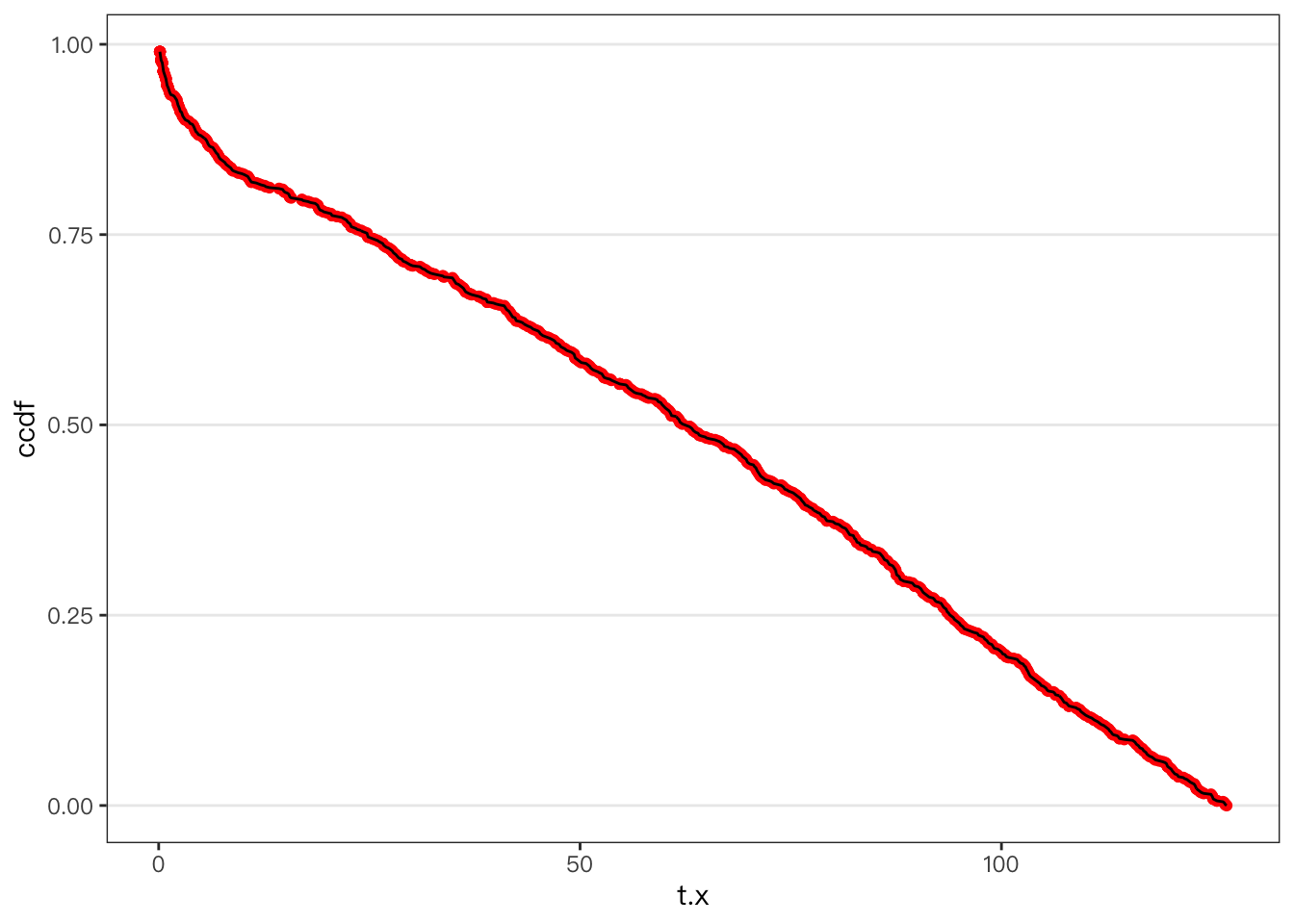
Note that t.x is the Time between first and last transactions. This is the “observed” part of lifetime. Let’s look at the distribution of t.x.
dtmp <- dcbs %>%
  # remove single purchase customers
  filter(t.x > 0) %>%
  # get value of cdf, P(X <= x)
  mutate(cdf = ecdf(t.x)(t.x)) %>%
  # get ccef, P(X > x)
  mutate(ccdf = 1 - cdf)


dtmp %>%
  ggplot(aes(x = t.x, y = ccdf)) +
  geom_point(color = "red") +
  geom_line()