Learning Resource: Social Network Analysis

Summary of Concepts

See my notes in “Analyzing Social Media Networks with NodeXL: Insights from A Connected World” (Hansen et al. 2019), Chapter 3 Sections 3.1-3.5 (pages 31-42).

• Node: Represents an entity (e.g., individual, organization) within the network.

• Edge: Connects two nodes, symbolizing a relationship or interaction.

• Graph: The entire structure comprising nodes and edges.

• Degree: Number of connections for a node, with in-degree and out-degree in directed networks.

• Path: Sequence of edges linking two nodes.

• Centrality: Quantifies the importance of nodes.

  • Degree Centrality: Frequency of a node in the network.

  • Betweenness Centrality: Frequency of a node appearing on shortest paths between other nodes.

  • Closeness Centrality: Proximity of a node to all other nodes.

  • Eigenvector Centrality: Influence level of a node.

• Diameter: Longest shortest path within the network.

• Community: Nodes more densely connected to each other than to the rest of the network.

• Homophily: Tendency to connect with similar others.

• Structural Holes: Gaps offering strategic advantages in information flow.

• Social Capital: Benefits and resources accessible through social networks.

• Small-world Network: Characterized by short path lengths and high clustering.

• Scale-free Network: Features a power-law degree distribution with few highly connected nodes.

• Network Density: Proportion of actual connections to potential connections.

• Modularity: Strength of a network’s division into modules or communities.

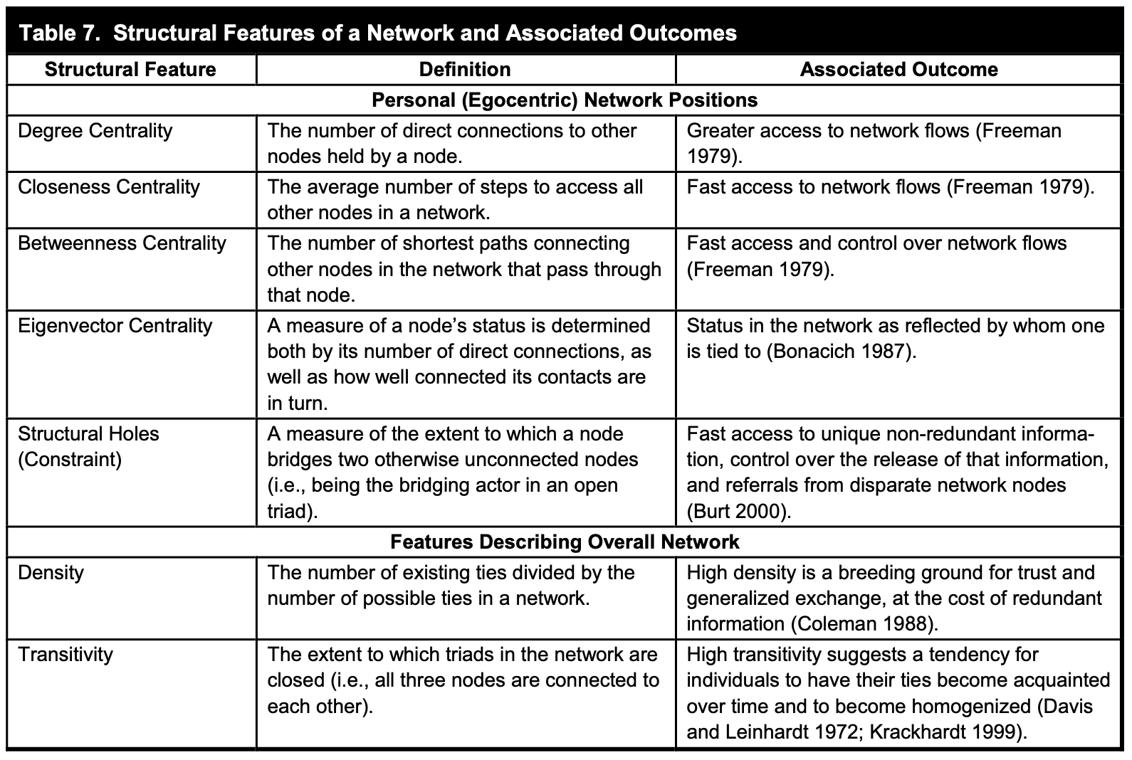
Summary Table

The following summary table is from (Kane et al. 2014).

Understanding the Role of Random Graphs in Network Analysis

• Contextual Analysis of Network Metrics:
  • Random graphs help in evaluating the significance of network metrics by providing a comparison point.
  • This approach determines if observed network patterns are typical or atypical under certain conditions.
• Assessing Significance and Likelihood:
  • By comparing real network characteristics to those of random graphs, it’s possible to assess the likelihood of these characteristics occurring by chance.
  • Significant differences in metrics like clustering suggest underlying social processes, not just random formation.
• Baseline for Comparison (Null Model):
  • A random graph acts as a baseline, representing a network where connections are formed randomly.
  • Comparing real networks to this baseline identifies non-random, significant features of the network.

• Simplicity in Modeling:
  • The simplest random graph mirrors the original graph in terms of number of nodes and density, facilitating easier statistical analysis.
• Methodological Rigor:
  • Utilizing random graphs adds rigor and depth to network analysis.
  • It aids in discerning meaningful social network patterns from those that might arise randomly.

This summary encapsulates the importance of using random graphs in social network analysis, particularly for understanding the significance and context of various network properties and metrics.

Datacamp course notes: key functions in igraph

Chapter 1: Basic Network Analysis

Creating and Visualizing Graphs

• Create Graph: graph.edgelist(as.matrix(df), directed = FALSE)
• Vertices and Edges: V(g), E(g)
• Graph Order and Size: gorder(g), gsize(g)
• Plot Graph: plot(g)

Attributes

• Add Vertex Attributes: set_vertex_attr(g, "attribute", value)
• Get Vertex Attributes: vertex_attr(g)
• Add Edge Attributes: set_edge_attr(g, "attribute", value)
• Get Edge Attributes: edge_attr(g)

Subsetting and Coloring

• Subsetting Networks: E(g)[[.inc('vertex')]], E(g)[[condition]]
• Coloring Vertices: V(g)$color <- ifelse(condition, "color1", "color2")

Layouts

• Graph Layouts: plot(g, layout = layout.fruchterman.reingold(g))

Chapter 2: Advanced Network Analysis Techniques

Directionality and Degrees

• Check Directionality: is.directed(g)
• Degree Analysis: degree(g, mode = c("out"))

Neighbors

• Identify Neighbors: neighbors(g, "vertex", mode = c("mode"))
• Common Neighbors: intersection(x, y)

Paths

• Longest Paths: farthest_vertices(g), get_diameter(g)
• Ego Networks: ego(g, N, 'vertex', mode=c('mode'))

Importance Measures

• Betweenness: betweenness(g, directed = TRUE, normalized = TRUE)
• Other Measures: degree, eigenvector centrality, closeness centrality, pagerank centrality

Chapter 3: Network Metrics and Random Graphs

Centrality and Density

• Eigenvector Centrality: eigen_centrality(g)$vector
• Network Density: edge_density(g)

Path Length and Random Graphs

• Average Path Length: mean_distance(g, directed = FALSE)
• Random Graphs: erdos.renyi.game(n, p.or.m, type)

Transitivity

• Transitivity: triangles(g), transitivity(g)
• Local Transitivity: transitivity(g, vids = 'vertex', type = "local")

Cliques

• Identifying Cliques: largest_cliques(g), max_cliques(g)

Chapter 4: Community Detection and Visualization

Assortativity and Reciprocity

• Assortativity: assortativity(g, values), assortativity.degree(g, directed = FALSE)
• Reciprocity: reciprocity(g)

Community Detection

• Fast-Greedy Detection: fastgreedy.community(g)
• Edge-Betweenness Detection: edge.betweenness.community(g)
• Community Analysis: length(x), sizes(x), membership(x), plot(x, g)

Visualization

• Visualization Packages: igraph, visNetwork, statnet, networkD3, ggnet, sigma, ggnetwork, rgexf, ggraph, threejs
• Threejs Visualization: library(threejs), graphjs(g)
• Adding Attributes: set_vertex_attr(g, "label", value = V(g)$name), set_vertex_attr(g, "color", value = "color")
• Coloring Communities: x = edge.betweenness.community(g), i <- membership(x), set_vertex_attr(g, "color", value = c("color1", "color2", "color3")[i]), graphjs(g)

Useful resource

• datacamp “Network Analysis in R”.

• YouTube tutorial Social Network Analysis: A Beginner’s Lab in R provided by Duke University Network Analysis Center.

• Textbook: “Statistical Analysis of Network Data with R” by Eric D. Kolaczyk (Kolaczyk and Csárdi 2014).

• Please check out R package: igraph. If you need to know how to compute a particular attribute of the network, the reference page is a good starting point.

• There are many packages available to make network plots. One very useful one is threejs which allows you to make interactive network visualizations. This package also integrates seamlessly with igraph.

Reference