Incorporating Time-Invariant Covariates into PNBD II
Introduction
In this post, we’ll continue discover the difference between the Cohort Modeling and the Extended PNBD Model with time-invariant covariates. Check here to see the previous post.
Data Prepare
First let’s import the transactional data, and select the customers who first purchase happened in 2017-2018.
trans_dat <- read_rds("~/Desktop/trans_dat.rds")

# select the customers who first purchase happened in 2017-2018
trans_dat <- trans_dat %>%
  filter(date <= as.Date("2019-12-31")) %>%
  filter(fp_yr <= 2018)

# glimpse
head(trans_dat)
## # A tibble: 6 × 4
##   cust  date        sales fp_yr
##   <chr> <date>      <dbl> <dbl>
## 1 10017 2018-03-08   674.  2018
## 2 10021 2017-08-27   495.  2017
## 3 10040 2017-05-13  2781   2017
## 4 10041 2018-07-21    72   2018
## 5 10048 2018-10-10  4472.  2018
## 6 10049 2017-02-05 18780   2017
summary(trans_dat)
##      cust                date                sales              fp_yr
##  Length:14943       Min.   :2017-01-01   Min.   :     0.5   Min.   :2017
##  Class :character   1st Qu.:2017-06-11   1st Qu.:   414.2   1st Qu.:2017
##  Mode  :character   Median :2018-02-16   Median :  1003.8   Median :2017
##                     Mean   :2018-04-08   Mean   :  2147.1   Mean   :2017
##                     3rd Qu.:2018-12-28   3rd Qu.:  2168.5   3rd Qu.:2018
##                     Max.   :2019-12-31   Max.   :476659.0   Max.   :2018
How many new customers joined the enterprise in 2017 and 2018?
trans_dat %>%
  group_by(fp_yr) %>%
  summarize(new_cust = n_distinct(cust))
## # A tibble: 2 × 2
##   fp_yr new_cust
##   <dbl>    <int>
## 1  2017     5114
## 2  2018     2767
Train/Test
-
Training: Two years, 2017-2018, transactional data.
-
Testing: One year, 2019, transactional data.
The Cohort Models
Cohort 2017
Prepare CLV data,
ch17_dat <- trans_dat %>%
  filter(fp_yr == 2017)

# build clv type of data
dclv_17 <- generate_clvdata(
  data = ch17_dat,
  splitDate = "2018-12-31"
)
## Note that: time unit is in < week >
Build PNBD Model,
m17 <- standard_PNBD_model(dclv_17)

# check
summary(m17)
## Pareto NBD Standard  Model
##
## Call:
## pnbd(clv.data = clvData, optimx.args = optimx.args)
##
## Fitting period:
## Estimation start  2017-01-01
## Estimation end    2018-12-31
## Estimation length 104.1429 Weeks
##
## Coefficients:
##       Estimate Std. Error  z-val Pr(>|z|)
## r      0.84155    0.08460  9.947  < 2e-16 ***
## alpha 54.31617    4.38954 12.374  < 2e-16 ***
## s      0.32609    0.03272  9.967  < 2e-16 ***
## beta   3.20325    1.06076  3.020  0.00253 **
## ---
## Signif. codes:  0 '***' 0.001 '**' 0.01 '*' 0.05 '.' 0.1 ' ' 1
##
## Optimization info:
## LL     -16587.4554
## AIC    33182.9107
## BIC    33209.0697
## KKT 1  TRUE
## KKT 2  TRUE
## fevals 409.0000
## Method Nelder-Mead
##
## Used Options:
## Correlation FALSE
Check the tracking plots,
plot(m17)
plot(m17, cumulative = TRUE)
On the testing period, the model curve is under the actual number of repeat transactions curve.
Cohort 2018
Similarly, we’ll get,
dclv_18 <- trans_dat %>%
  filter(fp_yr == 2018) %>%
  generate_clvdata(splitDate = "2018-12-31")
## Note that: time unit is in < week >
# model
m18 <- standard_PNBD_model(dclv_18)

# check model coef
summary(m18)
## Pareto NBD Standard  Model
##
## Call:
## pnbd(clv.data = clvData, optimx.args = optimx.args)
##
## Fitting period:
## Estimation start  2018-01-01
## Estimation end    2018-12-31
## Estimation length 52.0000 Weeks
##
## Coefficients:
##       Estimate Std. Error z-val Pr(>|z|)
## r      1.05005    0.30318 3.463 0.000533 ***
## alpha 40.98040   10.09464 4.060 4.92e-05 ***
## s      0.31008    0.04534 6.839 7.95e-12 ***
## beta   0.42186    0.22740 1.855 0.063572 .
## ---
## Signif. codes:  0 '***' 0.001 '**' 0.01 '*' 0.05 '.' 0.1 ' ' 1
##
## Optimization info:
## LL     -2529.2006
## AIC    5066.4012
## BIC    5090.1032
## KKT 1  TRUE
## KKT 2  TRUE
## fevals 285.0000
## Method Nelder-Mead
##
## Used Options:
## Correlation FALSE
Again, checking the tracking plots
plot(m18)
plot(m18, cumulative = TRUE)
On the testing period, the model curve is under the actual number of repeat transactions curve.
Interpret Model Coef
- The 2017 cohort has lower transaction rate and lower dropout rate comparing with the 2018-cohort.
| cohort | r | alpha | s | beta | lambda | mu |
|---|---|---|---|---|---|---|
| 2017 | 0.842 | 54.316 | 0.326 | 3.203 | 0.015 | 0.102 |
| 2018 | 1.050 | 40.980 | 0.310 | 0.422 | 0.026 | 0.735 |
Accuracy of Predictions
Let’s find the MAE and RMSE of the conditional expected transactions (CET) on the testing set.
| cohort | MAE | RMSE | Corr |
|---|---|---|---|
| 2017 | 0.431 | 0.924 | 0.517 |
| 2018 | 0.615 | 1.089 | 0.424 |
| All | 0.496 | 0.985 | 0.484 |
Let’s check the error distribution for cohort 2017,
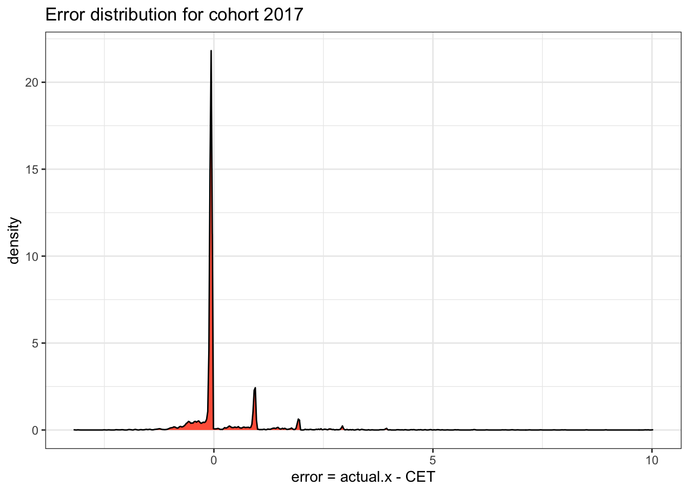
Why the customers purchased more in 2019, i.e. the actual transactions are larger than the model predictions?
After we talked with the company’s manger, we knew that the company started to perform a new membership service plan in 2019. The new service mode worked pretty well and leaded to the increasing number of repeat transactions.
The Extended PNBD Model
# set the fp_yr as a factor variable
trans_dat <- trans_dat %>%
  mutate(fp_yr = factor(fp_yr))

# check the factor level
levels(trans_dat$fp_yr)
## [1] "2017" "2018"
Note that, the model will use 2017 cohort as baseline or reference group.
# prepare static covariates data
static_cov_dat <- trans_dat %>%
  distinct(cust, fp_yr)

# clv data
dclv_all <- generate_clvdata(trans_dat, splitDate = "2018-12-31")
## Note that: time unit is in < week >
# make static covariates data as clv type of data
dclv_stat <- SetStaticCovariates(
  clv.data = dclv_all,
  data.cov.life = static_cov_dat,
  data.cov.trans = static_cov_dat,
  names.cov.life = "fp_yr",
  names.cov.trans = "fp_yr",
  name.id = "cust"
)
Now, we build the extended PNBD model with time-invariant covariates, which are fp_yr in this case.
ext_m <- standard_PNBD_model(
  dclv_stat,
  start.params.model = c(r = .88, alpha = 56.16, s = .29, beta = 2.25),
  start.params.life = c(fp_yr2018 = 2.01),
  start.params.trans = c(fp_yr2018 = .55)
)

# check the model
summary(ext_m)
## Pareto NBD with Static Covariates  Model
##
## Call:
## pnbd(clv.data = clvData, optimx.args = optimx.args, start.params.life = ..1,
##     start.params.trans = ..2)
##
## Fitting period:
## Estimation start  2017-01-01
## Estimation end    2018-12-31
## Estimation length 104.1429 Weeks
##
## Coefficients:
##                 Estimate Std. Error  z-val Pr(>|z|)
## r                0.86825    0.08145 10.660  < 2e-16 ***
## alpha           55.50864    4.28397 12.957  < 2e-16 ***
## s                0.31854    0.02583 12.332  < 2e-16 ***
## beta             2.90289    0.80920  3.587 0.000334 ***
## life.fp_yr2018   1.67367    0.29780  5.620 1.91e-08 ***
## trans.fp_yr2018  0.45153    0.10167  4.441 8.95e-06 ***
## ---
## Signif. codes:  0 '***' 0.001 '**' 0.01 '*' 0.05 '.' 0.1 ' ' 1
##
## Optimization info:
## LL     -19116.9873
## AIC    38245.9746
## BIC    38287.8079
## KKT 1  TRUE
## KKT 2  TRUE
## fevals 581.0000
## Method Nelder-Mead
##
## Used Options:
## Correlation     FALSE
## Regularization  FALSE
## Constraint covs FALSE
After checking the summary of the model, we know that the fp_yr affects both purchase process and attrition process (P-values are significant).
Now let’s check the tracking plot,
plot(ext_m)
plot(ext_m, cumulative = TRUE)
Interpret Model Coef
Since the 2017 cohort as the reference group, we already know its corresponding r, alpha, s, beta. However, we still need to calculate the alpha and beta for the 2018 cohort.
Plug into the formula: alpha = alpha0 * exp(-gamma1 * z1) and beta = beta0 * exp(-gamma2 * z2)
| cohort | r | alpha | s | beta | lambda | mu |
|---|---|---|---|---|---|---|
| 2017 | 0.868 | 55.509 | 0.319 | 2.903 | 0.016 | 0.110 |
| 2018 | 0.868 | 35.340 | 0.319 | 0.544 | 0.025 | 0.585 |
If we compare this model’s coefficients with the cohort models’, we’ll find the purchase/dropout rate estimates are quite similar for both models.
Accuracy of Predictions
Again, calculate the MAE and RMSE on CET.
ext_m_pred <- predict(ext_m) %>%
  select(cust = Id, actual.x, CET) %>%
  left_join(static_cov_dat)

ext_m_17_acc <- ext_m_pred %>%
  filter(fp_yr == 2017) %>%
  cal_err()

ext_m_18_acc <- ext_m_pred %>%
  filter(fp_yr == 2018) %>%
  cal_err()

ext_m_all_acc <- ext_m_pred %>%
  cal_err()

# result
bind_rows(ext_m_17_acc, ext_m_18_acc, ext_m_all_acc) %>%
  mutate(cohort = c(2017:2018, "All"), .before = 1) %>%
  mutate(across(where(is.numeric), round, digits = 3)) %>%
  print_kbl(
    cap = "Extended PNBD Model Error Measure on cohort 2017, 2018 and all together"
  )
| cohort | MAE | RMSE | Corr |
|---|---|---|---|
| 2017 | 0.432 | 0.924 | 0.517 |
| 2018 | 0.615 | 1.085 | 0.429 |
| All | 0.496 | 0.983 | 0.486 |
Conclusion
Comparing the prediction error of two models, we find that two models prediction behaviors are very close. I prefer the extended PNBD model for this data.