Incorporating Time-Invariant Covariates into PNBD
Introducton
The original Pareto-NBD Model is awesome, but it does not allow us to add any covariates. In some cases, the covariates may affect the purchase, or the attrition process, or both. In this post, we will learn the simple case, adding the time-invariant covariates using CLVTools R package📦 and my own zetaclv package.
Next, we will predict customer’s future transactions using two approaches:
-
Divide the customers into different cohort groups, which is defined by the
first purchase year, then build the models for each cohort. -
Without “cohorting” the customer, we’ll build a model using the
first purchase yearas time-invariant covariates.
After that, let’s compare and understand the difference between two models/approaches, and choose the better one.
Add Time-Invariant Covariates in PNBD
If you familiar with the original Pareto-NBD Model (here to review), then this new model is not complicated at all!
Recall that, in PNBD Model, we assume that the transactional rate, $\lambda$, and the dropout rate, $\mu$, have the following distribution $$\lambda \sim \text{Gamma}(r, \alpha), \ \ \mu \sim \text{Gamma}(s, \beta)$$
We keep the shape parameters (i.e. $r, s$) unchanged, but replace the following scale parameters:
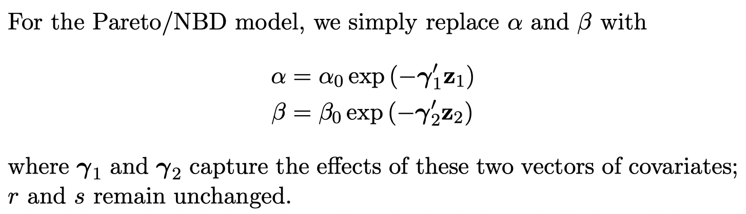
For more details, see Fader PS, Hardie BGS (2007). “Incorporating time-invariant covariates into the Pareto/NBD and BG/NBD models.”
Why we set $\alpha, \beta$ in this form?
The idea is from proportional hazard model (check my previous post if needed).
-
$\alpha_0, \beta_0$ refer baseline hazard.
-
The $\gamma$ part refers the log of hazard ratio.
Data Prepare
The transactional data has cust, date and sales information.
# add first purchase year column
dat <- eg_trans_data %>%
  with_groups(
    .groups = cust,
    .f = mutate,
    # first purchase year
    fp_yr = min(lubridate::year(date))
  ) %>%
  filter(fp_yr < 2020) %>%
  arrange(cust, date)

# have a look
head(dat, 5) %>% print_kbl(cap = "dat")
| cust | date | sales | fp_yr |
|---|---|---|---|
| uid0001 | 2019-12-02 | 3470 | 2019 |
| uid0001 | 2020-04-20 | 1050 | 2019 |
| uid0001 | 2020-04-20 | 124 | 2019 |
| uid0003 | 2018-12-11 | 1948 | 2018 |
| uid0003 | 2019-02-22 | 828 | 2018 |
summary(dat)
##       cust            date                sales           fp_yr
##  uid3414:  248   Min.   :2018-01-11   Min.   :    0   Min.   :2018
##  uid0384:  239   1st Qu.:2019-01-26   1st Qu.:  182   1st Qu.:2018
##  uid1156:  191   Median :2019-08-01   Median :  560   Median :2018
##  uid1149:  173   Mean   :2019-09-22   Mean   : 1431   Mean   :2018
##  uid0018:  155   3rd Qu.:2020-05-14   3rd Qu.: 1465   3rd Qu.:2019
##  uid3466:  152   Max.   :2021-06-07   Max.   :79270   Max.   :2019
##  (Other):21307
We will use the fp_yr variable to define the cohort group. How many customers in each cohort?
dat %>%
  group_by(fp_yr) %>%
  summarize(n_cust = n_distinct(cust))
## # A tibble: 2 × 2
##   fp_yr n_cust
##   <dbl>  <int>
## 1  2018   1097
## 2  2019   2314
Cohort Models
Cohort data:
# cohort data
dat18 <- filter(dat, fp_yr == 2018)
dat19 <- filter(dat, fp_yr == 2019)
Build the clv type of data:
dclv_18 <- generate_clvdata(
  data = dat18,
  splitDate = "2019-12-31"
)
## Note that: time unit is in < week >
dclv_18
## CLV Transaction Data
##
## Call:
## clvdata(data.transactions = data, date.format = "ymd", time.unit = timeUnit,
##     estimation.split = splitDate, name.id = "cust", name.date = "date",
##     name.price = "sales")
##
## Total # customers    1097
## Total # transactions 4968
## Spending information TRUE
##
##
## Time unit         Weeks
##
## Estimation start  2018-01-11
## Estimation end    2019-12-31
## Estimation length 102.7143 Weeks
##
## Holdout start     2020-01-01
## Holdout end       2021-06-07
## Holdout length    74.71429 Weeks
dclv_19 <- generate_clvdata(
  data = dat19,
  splitDate = "2019-12-31"
)
## Note that: time unit is in < week >
dclv_19
## CLV Transaction Data
##
## Call:
## clvdata(data.transactions = data, date.format = "ymd", time.unit = timeUnit,
##     estimation.split = splitDate, name.id = "cust", name.date = "date",
##     name.price = "sales")
##
## Total # customers    2314
## Total # transactions 5108
## Spending information TRUE
##
##
## Time unit         Weeks
##
## Estimation start  2019-01-01
## Estimation end    2019-12-31
## Estimation length 52.0000 Weeks
##
## Holdout start     2020-01-01
## Holdout end       2021-06-07
## Holdout length    74.71429 Weeks
Now, let’s model the cohort group data:
m18 <- standard_PNBD_model(dclv_18)

summary(m18)
## Pareto NBD Standard  Model
##
## Call:
## pnbd(clv.data = clvData, optimx.args = optimx.args)
##
## Fitting period:
## Estimation start  2018-01-11
## Estimation end    2019-12-31
## Estimation length 102.7143 Weeks
##
## Coefficients:
##       Estimate Std. Error  z-val Pr(>|z|)
## r      0.39734    0.04020  9.884  < 2e-16 ***
## alpha 10.74518    1.01108 10.627  < 2e-16 ***
## s      0.12227    0.03574  3.421 0.000623 ***
## beta   2.79356    2.84873  0.981 0.326774
## ---
## Signif. codes:  0 '***' 0.001 '**' 0.01 '*' 0.05 '.' 0.1 ' ' 1
##
## Optimization info:
## LL     -8303.6317
## AIC    16615.2633
## BIC    16635.2647
## KKT 1  TRUE
## KKT 2  TRUE
## fevals 195.0000
## Method Nelder-Mead
##
## Used Options:
## Correlation FALSE
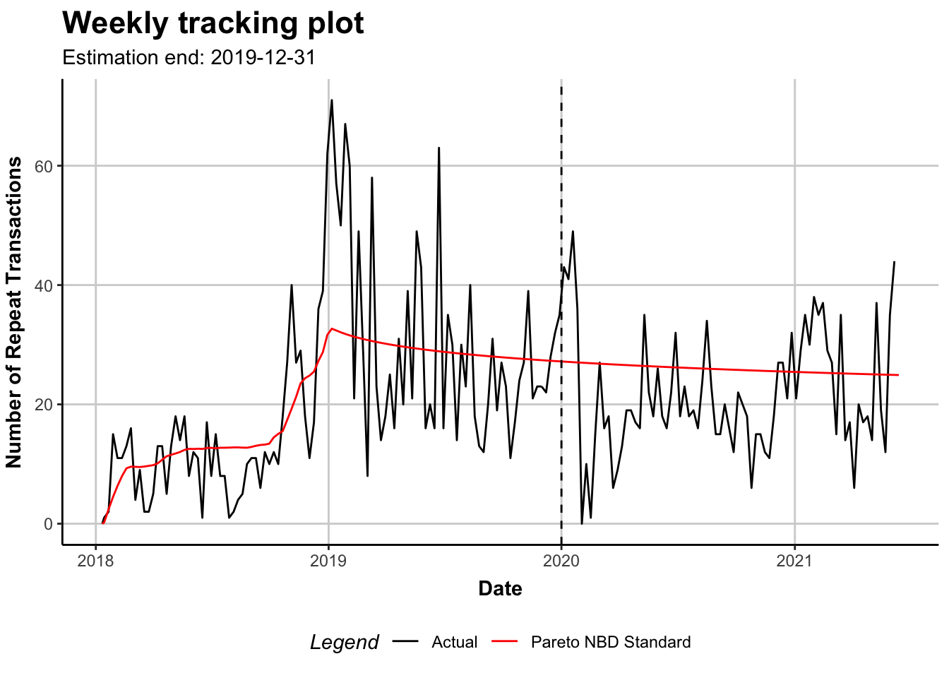
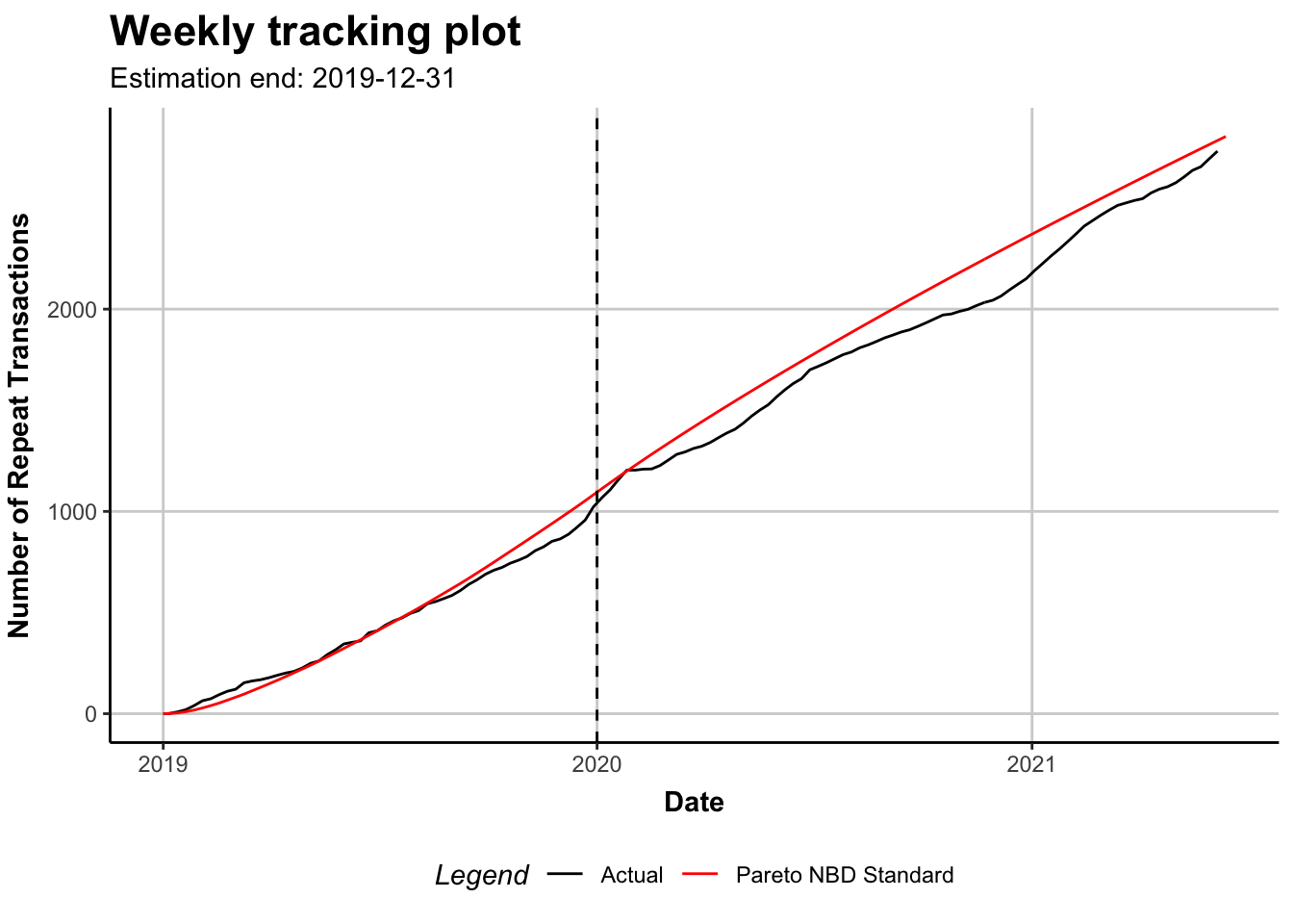
plot(m18)
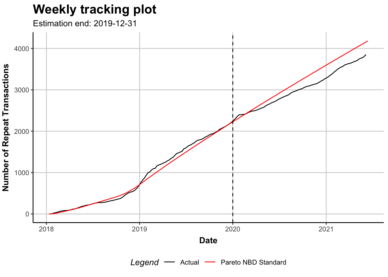
plot(m18, cumulative = TRUE)
m19 <- standard_PNBD_model(dclv_19)

summary(m19)
## Pareto NBD Standard  Model
##
## Call:
## pnbd(clv.data = clvData, optimx.args = optimx.args)
##
## Fitting period:
## Estimation start  2019-01-01
## Estimation end    2019-12-31
## Estimation length 52.0000 Weeks
##
## Coefficients:
##       Estimate Std. Error z-val Pr(>|z|)
## r      0.44721    0.06257 7.148 8.82e-13 ***
## alpha 15.02084    1.76408 8.515  < 2e-16 ***
## s      0.26878    0.04008 6.706 1.99e-11 ***
## beta   1.08620    0.56096 1.936   0.0528 .
## ---
## Signif. codes:  0 '***' 0.001 '**' 0.01 '*' 0.05 '.' 0.1 ' ' 1
##
## Optimization info:
## LL     -4778.1858
## AIC    9564.3715
## BIC    9587.3584
## KKT 1  TRUE
## KKT 2  TRUE
## fevals 489.0000
## Method Nelder-Mead
##
## Used Options:
## Correlation FALSE
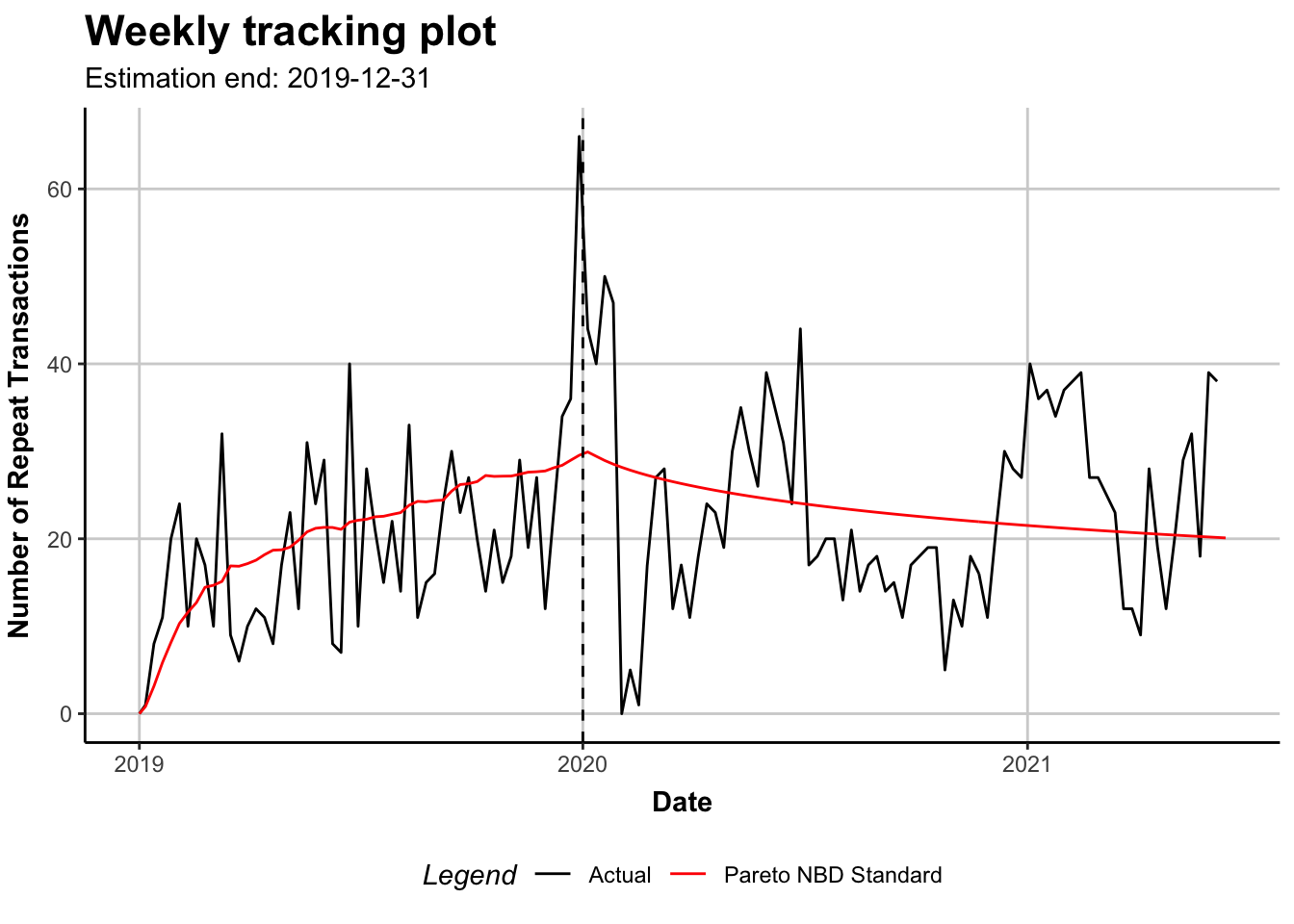
plot(m19)
plot(m19, cumulative = TRUE)
compare the model coefficients:
cohort_model_coefs <- rbind(`2018` = coef(m18), `2019` = coef(m19))

cohort_model_coefs %>%
  as_tibble(rownames = "cohort") %>%
  print_kbl("compare the model's coef from different cohort")
| cohort | r | alpha | s | beta |
|---|---|---|---|---|
| 2018 | 0.3973431 | 10.74518 | 0.1222724 | 2.793557 |
| 2019 | 0.4472133 | 15.02084 | 0.2687787 | 1.086205 |
Interpret Coef
The expected value of transaction rate lambda is r/alpha, and the expected value of dropout rate mu is s/beta.
cohort_model_coefs %>%
  as_tibble(rownames = "cohort") %>%
  mutate(lambda = r / alpha, mu = s / beta) %>%
  mutate(across(c(r:mu), round, digits = 3)) %>%
  print_kbl("compare transaction/dropout rate")
| cohort | r | alpha | s | beta | lambda | mu |
|---|---|---|---|---|---|---|
| 2018 | 0.397 | 10.745 | 0.122 | 2.794 | 0.037 | 0.044 |
| 2019 | 0.447 | 15.021 | 0.269 | 1.086 | 0.030 | 0.247 |
We can conclude that the 2018-cohort has higher purchase rate and lower dropout rate.
Extended PNBD Model
The clv type of data:
dclv_all <- generate_clvdata(
  data = dat,
  splitDate = "2019-12-31"
)
## Note that: time unit is in < week >
dclv_all
## CLV Transaction Data
##
## Call:
## clvdata(data.transactions = data, date.format = "ymd", time.unit = timeUnit,
##     estimation.split = splitDate, name.id = "cust", name.date = "date",
##     name.price = "sales")
##
## Total # customers    3411
## Total # transactions 10076
## Spending information TRUE
##
##
## Time unit         Weeks
##
## Estimation start  2018-01-11
## Estimation end    2019-12-31
## Estimation length 102.7143 Weeks
##
## Holdout start     2020-01-01
## Holdout end       2021-06-07
## Holdout length    74.71429 Weeks
The static covariate data:
stat_cov <- dat %>%
  distinct(cust, fp_yr) %>%
  mutate(fp_yr = factor(fp_yr, levels = c(2018, 2019)))

summary(stat_cov)
##       cust       fp_yr
##  uid0001:   1   2018:1097
##  uid0003:   1   2019:2314
##  uid0004:   1
##  uid0005:   1
##  uid0006:   1
##  uid0008:   1
##  (Other):3405
The clv type of covariate data:
dclv_stat <- SetStaticCovariates(
  clv.data = dclv_all,
  data.cov.life = stat_cov,
  data.cov.trans = stat_cov,
  names.cov.life = "fp_yr",
  names.cov.trans = "fp_yr",
  name.id = "cust"
)

dclv_stat
## CLV Transaction Data with Static Covariates
##
## Call:
## clvdata(data.transactions = data, date.format = "ymd", time.unit = timeUnit,
##     estimation.split = splitDate, name.id = "cust", name.date = "date",
##     name.price = "sales")
##
## Total # customers    3411
## Total # transactions 10076
## Spending information TRUE
##
##
## Time unit         Weeks
##
## Estimation start  2018-01-11
## Estimation end    2019-12-31
## Estimation length 102.7143 Weeks
##
## Holdout start     2020-01-01
## Holdout end       2021-06-07
## Holdout length    74.71429 Weeks
##
## Covariates
## Trans. Covariates    fp_yr2019
##        # covs        1
## Life.  Covariates    fp_yr2019
##        # covs        1
The PNBD Model with time-invariant covariates:
ext_m <- standard_PNBD_model(dclv_stat)

summary(ext_m)
## Pareto NBD with Static Covariates  Model
##
## Call:
## pnbd(clv.data = clvData, optimx.args = optimx.args)
##
## Fitting period:
## Estimation start  2018-01-11
## Estimation end    2019-12-31
## Estimation length 102.7143 Weeks
##
## Coefficients:
##                 Estimate Std. Error  z-val Pr(>|z|)
## r                0.38211    0.02952 12.945  < 2e-16 ***
## alpha            9.36586    0.84549 11.077  < 2e-16 ***
## s                0.16033    0.03288  4.877 1.08e-06 ***
## beta             2.87077    2.27740  1.261   0.2075
## life.fp_yr2019   1.19338    0.58044  2.056   0.0398 *
## trans.fp_yr2019 -0.52757    0.11754 -4.489 7.17e-06 ***
## ---
## Signif. codes:  0 '***' 0.001 '**' 0.01 '*' 0.05 '.' 0.1 ' ' 1
##
## Optimization info:
## LL     -13095.4075
## AIC    26202.8149
## BIC    26239.6235
## KKT 1  TRUE
## KKT 2  TRUE
## fevals 607.0000
## Method Nelder-Mead
##
## Used Options:
## Correlation     FALSE
## Regularization  FALSE
## Constraint covs FALSE
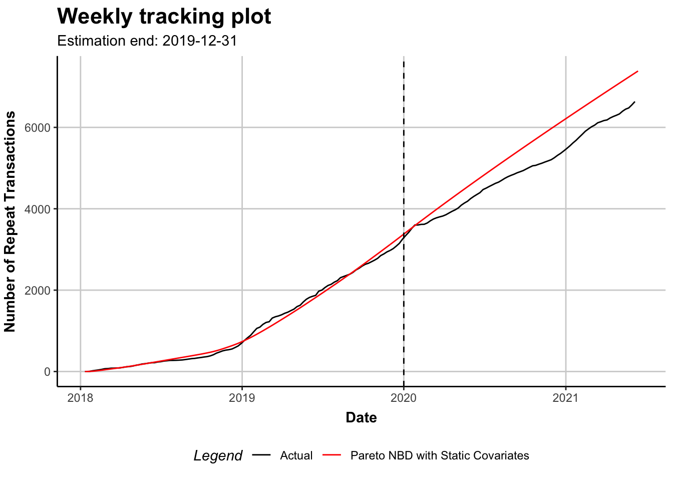
plot(ext_m, cumulative = TRUE)
Interpret Coef
coef(ext_m) %>%
  enframe(name = "coef")
## # A tibble: 6 × 2
##   coef             value
##   <chr>            <dbl>
## 1 r                0.382
## 2 alpha            9.37
## 3 s                0.160
## 4 beta             2.87
## 5 life.fp_yr2019   1.19
## 6 trans.fp_yr2019 -0.528
Note that, the baseline or “reference group” is cohort-2018, and we already know its 4 parameters.
For cohort-2019,
-
The cohort-2018 and cohort-2019 share the same values of
rands. -
We only need to find its
alphaandbeta.
Plug into the formula: alpha = alpha0 * exp(-gamma1 * z1) and beta = beta0 * exp(-gamma2 * z2)
coefs <- unname(coef(ext_m))

# for cohort-2018, as reference group
r <- coefs[1]
s <- coefs[3]
alpha0 <- coefs[2]
beta0 <- coefs[4]

# here, the covariates are indicator variables (0/1; 0 refers baseline)
z1 <- 1
z2 <- 1

# gamma
gamma1 <- coefs[6]
gamma2 <- coefs[5]

# for cohort-2019
alpha <- alpha0 * exp(-gamma1 * z1)
beta <- beta0 * exp(-gamma2 * z2)

# put all together
coef_tbl <- tibble(
  r = c(r, r),
  alpha = c(alpha0, alpha),
  s = c(s, s),
  beta = c(beta0, beta)
) %>%
  mutate(cohort = c(2018, 2019), .before = 1) %>%
  mutate(
    lambda = r / alpha,
    mu = s / beta
  )
coef_tbl %>%
  mutate(across(r:mu, round, digits = 3)) %>%
  print_kbl(
    highlight_cols = c("lambda", "mu"),
    cap = "compare transaction/dropout rate"
  )
| cohort | r | alpha | s | beta | lambda | mu |
|---|---|---|---|---|---|---|
| 2018 | 0.382 | 9.366 | 0.16 | 2.871 | 0.041 | 0.056 |
| 2019 | 0.382 | 15.873 | 0.16 | 0.870 | 0.024 | 0.184 |
Compare Two Models
The following tables show the values of coefficients from two models:
| cohort | r | alpha | s | beta | lambda | mu |
|---|---|---|---|---|---|---|
| 2018 | 0.397 | 10.745 | 0.122 | 2.794 | 0.037 | 0.044 |
| 2019 | 0.447 | 15.021 | 0.269 | 1.086 | 0.030 | 0.247 |
| cohort | r | alpha | s | beta | lambda | mu |
|---|---|---|---|---|---|---|
| 2018 | 0.382 | 9.366 | 0.16 | 2.871 | 0.041 | 0.056 |
| 2019 | 0.382 | 15.873 | 0.16 | 0.870 | 0.024 | 0.184 |
According to above results, both Cohort Model and Extended PNBD Model have the same conclusion that cohort-2018 is better, which has the higher purchase rate and lower dropout rate.
The time unit used in the models is week. Now let’s change the time unit to year and try to get more intuitive result (i.e. compare the average number of transactions in a year, lambda, etc.).
| cohort | lambda | mu |
|---|---|---|
| 2018 | 1.92 | 2.28 |
| 2019 | 1.55 | 12.87 |
| cohort | lambda | mu |
|---|---|---|
| 2018 | 2.12 | 2.90 |
| 2019 | 1.25 | 9.58 |
Compare Prediction Accuracy
Now let’s compare two models’ prediction error for CET (conditional expected transactions).
-
CET = PAlive * updated mean of Pareto/NBD
-
The value of CET has already involved the probability of alive (PAlive)!
ext_pred <- predict(ext_m)

ext_err <- ext_pred %>%
  summarize(
    MAE = mean(abs(actual.x - CET)),
    RMSE = sqrt(mean((actual.x - CET)^2))
  )
ch18_pred <- predict(m18) %>%
  select(actual.x, CET)

ch19_pred <- predict(m19) %>%
  select(actual.x, CET)

ch_err <- bind_rows(ch18_pred, ch19_pred) %>%
  summarize(
    MAE = mean(abs(actual.x - CET)),
    RMSE = sqrt(mean((actual.x - CET)^2))
  )
bind_rows(
  ch_err,
  ext_err
) %>%
  mutate(type = c("cohort model", "ext PNBD"), .before = 1) %>%
  print_kbl(cap = "Compare Model Prediction Error")
| type | MAE | RMSE |
|---|---|---|
| cohort model | 1.031840 | 2.585261 |
| ext PNBD | 1.070709 | 2.623130 |
In this case, the cohort model is slightly more accurate in terms of MAE and RMSE.
However, in practice we may deal with many cohort groups and thus have to build many models. At that time, the extended PNBD with time-invariant covariate may save you a lot of time.
For example, in the above story, we used the first purchase year as time-invariant covariates to build ONLY ONE model instead of building m18 and m19, 2 separate models for 2018/2019 cohort groups.
Of course, there is no free lunch. We always need to balance the degree of “convenience” and the prediction accuracy.
Reference
-
Fader PS, Hardie BGS (2007). “Incorporating time-invariant covariates into the Pareto/NBD and BG/NBD models.” URL http://www.brucehardie.com/notes/019/time_invariant_covariates.pdf.