CLV Prediction in R
Introduction
In the previous posts, we talked about the theoretical part of Pareto/NBD model. This time, we will go over the CLV prediction in R.
Customer lifetime value (CLV) is a huge topic and CLV prediction is super important for the retailers. The decision maker could use CLV to determine “who” is the best customer and get ready to target them.
Roughly speaking,
$$ CLV \approx \text{future num of transactions} \cdot \text{future average spending} $$-
apply the Pareto/NBD model to predict the future # of transactions
-
apply the Gamma-Gamma model to predict the future average spending
This approach is a more probabilistic approach. Of course, we can use machine learning (tree based models) to predict the future total spending, say during next year, using tidymodels workflow, but personally I prefer the simple but powerful probability models.
R package
I mainly use the following 3 R package to fulfill the CLV task:
CLVTools is pretty comprehensive and powerful over all 3. BTYDPlus provides lots of extensions for BTYD, for example its MBG/NBD model fixed the limitation of the BG/BD. BTYD is the oldest one but good for learning propose.
library(zetaEDA)
library(zetaclv)
library(BTYD)
library(BTYDplus)
enable_zeta_ggplot_theme()
Import the fake transactional data for this tutorial,
cohort19 <- eg_trans_data %>%
  # add column first purchase year
  with_groups(cust, mutate, fp_yr = min(lubridate::year(date))) %>%
  filter(fp_yr == 2019) %>%
  select(-fp_yr)

# have a look
cohort19 %>%
  head() %>%
  arrange(cust, date) %>%
  print_kbl(cap = "Cohort 2019 transaction data")
| cust | date | sales |
|---|---|---|
| uid0001 | 2019-12-02 | 3470 |
| uid0001 | 2020-04-20 | 1050 |
| uid0001 | 2020-04-20 | 124 |
| uid0005 | 2019-08-08 | 1169 |
| uid0006 | 2019-04-20 | 508 |
| uid0006 | 2020-04-09 | 922 |
Build the Pareto/NBD Model using CLVTools 📦.
# build clv class of data
dclv <- generate_clvdata(
  data = cohort19,
  timeUnit = "week",
  splitDate = NULL
)
## Note that: time unit is in < week >
# model object
pareto_nbd <- pnbd(dclv)

summary(pareto_nbd)
## Pareto NBD Standard  Model
##
## Call:
## pnbd(clv.data = dclv)
##
## Fitting period:
## Estimation start  2019-01-01
## Estimation end    2021-06-07
## Estimation length 126.8571 Weeks
##
## Coefficients:
##       Estimate Std. Error  z-val Pr(>|z|)
## r      0.45945    0.04783  9.606   <2e-16 ***
## alpha 20.06906    1.71733 11.686   <2e-16 ***
## s      0.18148    0.01842  9.853   <2e-16 ***
## beta   1.01572    0.44456  2.285   0.0223 *
## ---
## Signif. codes:  0 '***' 0.001 '**' 0.01 '*' 0.05 '.' 0.1 ' ' 1
##
## Optimization info:
## LL     -12872.0449
## AIC    25752.0898
## BIC    25775.0767
## KKT 1  TRUE
## KKT 2  TRUE
## fevals 24.0000
## Method L-BFGS-B
##
## Used Options:
## Correlation FALSE
All these packages have common modeling steps, which will be showed in the next section.
Build cbs data
(C)ustomer-(B)y-(S)ufficient data includes:
-
x: number of repeat transactions.-
Usually, multiple transactions on the same day just count once; in other words, count the how many purchase days.
-
同一天多次购买,算一次。一般来说,是计数多少个不同的购买日期。
-
-
t.x: Time between first and last transactions.- 首次购买 至 最后一次购买 相隔的时间。
-
T.cal: Time between first transaction and end of calibration period.- 首次购买 至 当前观测日 相隔的时间。
More details for the cbs data, check this:
# the help doc explains all above variables
?BTYDplus::elog2cbs()
We have many ways to get cbs data from transactional data, here I use my own function.
cbs_dat <- generate_cbs(
  data = cohort19,
  timeUnit = "week",
  splitDate = NULL
) %>%
  select(cust, x, t.x, T.cal)
## Note that: time unit is in < week >
# check
cbs_dat %>%
  head() %>%
  print_kbl(cap = "example: CBS data")
| cust | x | t.x | T.cal |
|---|---|---|---|
| uid0001 | 1 | 20.00000 | 79.00000 |
| uid0005 | 0 | 0.00000 | 95.57143 |
| uid0006 | 1 | 50.71429 | 111.28571 |
| uid0010 | 0 | 0.00000 | 120.42857 |
| uid0011 | 0 | 0.00000 | 124.85714 |
| uid0012 | 0 | 0.00000 | 87.00000 |
Predict PAlive
This is the most tough part w.r.t computation in Pareto/NBD modeling. If you forget the story, please check my previous post here.
Result from “A Note on Deriving the Pareto/NBD Model and Related Expressions” shows that:
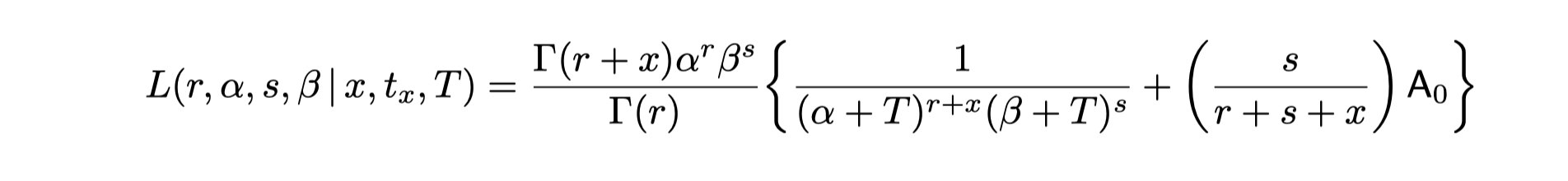
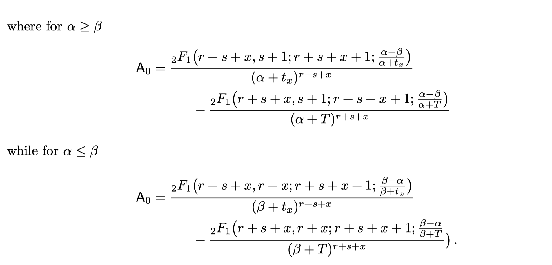

Checking source code
If we check the source code of the following functions, we’ll find they apply the above formula to get the probability of alive.
# check the source code:

# BTYD::pnbd.PAlive()

# BTYD::pnbd.generalParams
After checking, you will find that BTYD::pnbd.PAlive() internally called BTYD::pnbd.generalParams .
Insight
The probability of alive (PALive) for a given customer is a function of:
-
The 4 model parameters $ (r, \alpha, s, \beta) $.
-
The customer’s own CBS info, $ (x, t_x, T) $.
To sum up,
- PAlive is a function of 4 parameters and individual’s CBS data.
$$ \text{PAlive} = \text{function}(r, \alpha, s, \beta, x, t_x, T) $$
- PAlive DOES NOT depend on the prediction horizon $t $ ! This is a common mistake when someone explains this prediction result.
Interpretation
Let’s find the PAlive for cust:uid0001 who had x=1 repeat transactions (or 2 transactions in total),
# his own cbs
cbs_dat %>%
  filter(cust == "uid0001")
##      cust x t.x T.cal
## 1 uid0001 1  20    79
# palive is a function of 4 model params and his own cbs
palive_val <- BTYD::pnbd.PAlive(
  params = unname(coef(pareto_nbd)),
  x = 1,
  t.x = 20,
  T.cal = 79
)

palive_val
## [1] 0.6198724
For customer uid0001, the probability that he is still “alive” at present (i.e. $ \tau > T $ ) is 62.0%. In other words, there is 38.0% chance that the customer uid0001 had already leaved the company.
What about the customers with single purchase?
single_cbs_dat <- cbs_dat %>%
  filter(x == 0) %>%
  arrange(T.cal)

single_cbs_dat %>%
  head() %>%
  print_kbl(cap = "Example of the single purchase cbs data")
| cust | x | t.x | T.cal |
|---|---|---|---|
| uid2509 | 0 | 0 | 74.85714 |
| uid3443 | 0 | 0 | 74.85714 |
| uid4183 | 0 | 0 | 74.85714 |
| uid0301 | 0 | 0 | 75.00000 |
| uid0727 | 0 | 0 | 75.00000 |
| uid0799 | 0 | 0 | 75.00000 |
single_ids <- single_cbs_dat$cust

# use predict in clvtools to get all prediction results
all_preds <- predict(pareto_nbd, prediction.end = 52)

# discover the ones with single purchase
plotdata <- all_preds %>%
  filter(Id %in% single_ids) %>%
  select(Id, PAlive) %>%
  left_join(single_cbs_dat, by = c("Id" = "cust")) %>%
  arrange(T.cal)

# have a look
plotdata %>%
  head() %>%
  print_kbl(cap = "Example of palive for the one with single purchase")
| Id | PAlive | x | t.x | T.cal |
|---|---|---|---|---|
| uid2509 | 0.3266206 | 0 | 0 | 74.85714 |
| uid3443 | 0.3266206 | 0 | 0 | 74.85714 |
| uid4183 | 0.3266206 | 0 | 0 | 74.85714 |
| uid0301 | 0.3263572 | 0 | 0 | 75.00000 |
| uid0727 | 0.3263572 | 0 | 0 | 75.00000 |
| uid0799 | 0.3263572 | 0 | 0 | 75.00000 |
plotdata %>%
  ggplot(aes(x = T.cal, y = PAlive)) +
  geom_jitter(alpha = .2, size = 2.5, width = .42) +
  geom_line(color = "tomato", size = 1.4) +
  labs(
    x = "T.cal (unit: week)",
    title = "PAlive (of single purchase customers) as a function of T.cal"
  )
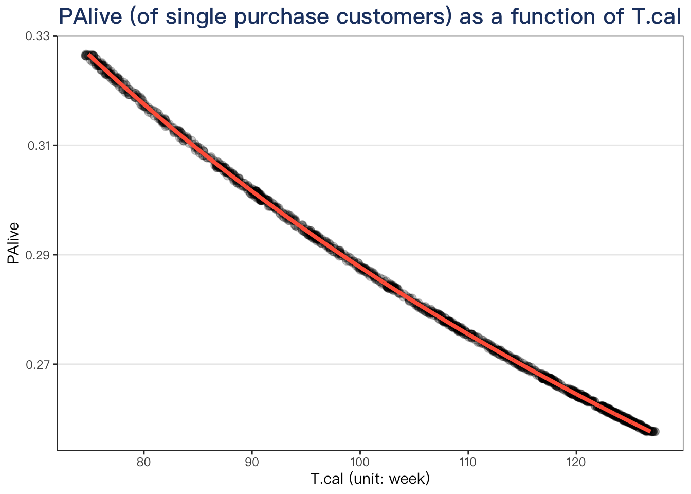
If the customer had only 1 purchase, the earlier the purchase made, the more likely he will drop out. Fits our intuition.
Predict Conditional Expected Transaction
Insight
From last post, we have showed the Conditional Expected Transaction, CET, is the product of PAlive and the updated mean of Pareto/NBD:
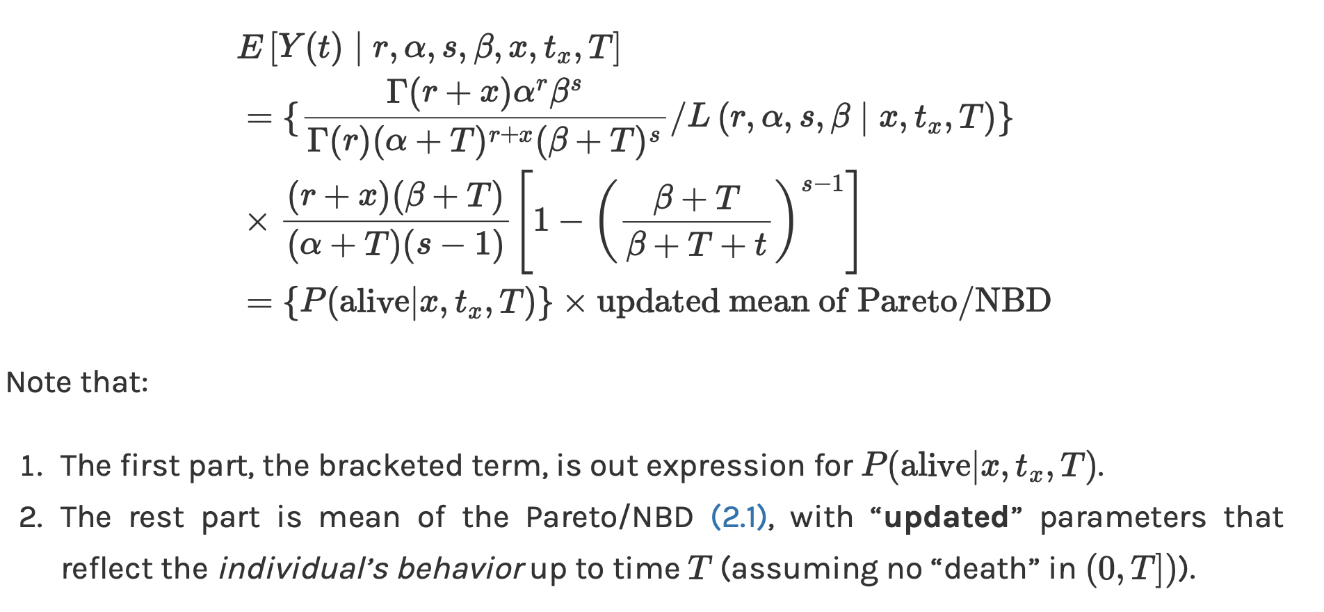
-
CET = PAlive * updated mean of Pareto/NBD
-
The value of CET has already involved the probability of alive (PAlive)!
Example
Let’s check it by manually calculate the CET for the future 52 weeks.
params <- unname(coef(pareto_nbd))

# model parameters
r = params[1]
a = params[2]
s = params[3]
b = params[4]

# the customers cbs
cbs_dat %>%
  filter(cust == "uid0001")
##      cust x t.x T.cal
## 1 uid0001 1  20    79
Setting inputs,
# note that from above formula 't.x' is not needed for the updated mean
x = 1
Tcal = 79

# prediction time horizon
t = 52
# follow the formula to compute updated mean of pnbd
part1 <- (r+x)*(b+Tcal)
part2 <- (a+Tcal)*(s-1)
part3 <- 1 - ((b+Tcal)/(b+Tcal+t))^(s-1)

updated_mean <- part1/part2*part3

updated_mean
## [1] 0.7295102
t.x, only involves x and Tcal of the individual.
-
The individual’s
t.xhas nothing to do with “updated” mean of Pareto/NBD. This is a interesting point! -
However, individual’s
t.xdefinitely affects the PAlive.
# CET calculated manually
updated_mean * palive_val
## [1] 0.4522032
# CET calculated using BTYD
BTYD::pnbd.ConditionalExpectedTransactions(
  params = params,
  T.star = 52,
  x = 1,
  t.x = 20,
  T.cal = 79
)
## [1] 0.4522032
# CET calculated using CLVTools
all_preds %>%
  select(Id, CET) %>%
  filter(Id == "uid0001") %>%
  pull(CET)
## [1] 0.4522032
Oh yeah, all the above results are the same 🙂.
What happened on “updated” mean of Pareto/NBD?
# mean of Pareto/NBD
# without the individual level information
mean_pnbd <- BTYD::pnbd.Expectation(params = params, t = 52)
mean_pnbd
## [1] 0.6949746
# updated mean of Pareto/NBD
# for customer uid0001
updated_mean
## [1] 0.7295102
After updating the parameter with the individual’s behavior, we can see the “new mean” increase a little bit from 0.695 to 0.73.
Interpreation
Under customer uid0001’s past behavior, i.e. given his cbs data, the model expects he will make 0.45 number of transactions in the future 52 weeks.
Predict Average Spending
Insight
We will predict the customer’s future average spending using Gamma-Gamma-Model (if you don’t remember the story, click it). We have showed that ,
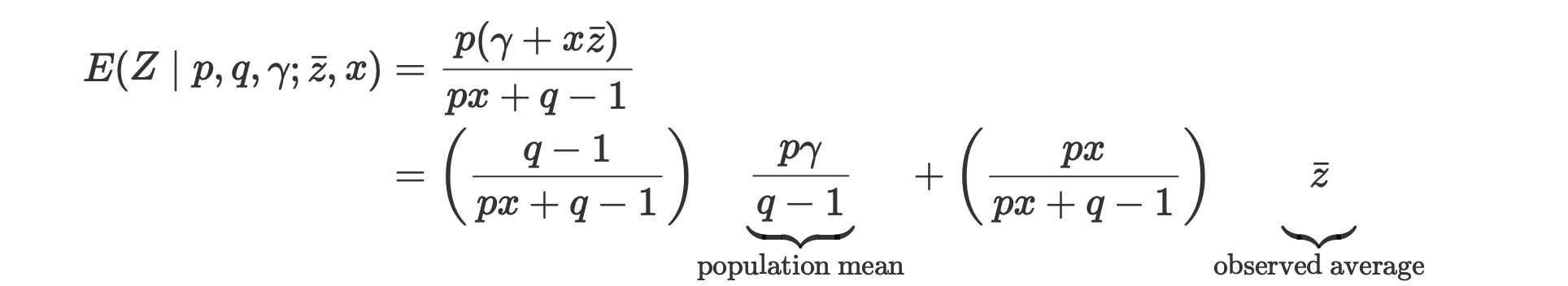
The moral of the story is that:
-
If the customer has many transactions, then his own average spending “will say more”, and the population mean “will say less”.
-
On the other hand, if the customer has a small number of transactions, then the population mean “will say more” on his future average spending.
Parameter Estimation (including the 1st trans.)
spend_cbs_data <- generate_cbs(
  data = cohort19,
  timeUnit = "week",
  splitDate = NULL
) %>%
  # total number of tran
  mutate(num_trans = x + 1) %>%
  # average spending
  mutate(avg_spend = sales/num_trans) %>%
  mutate(is_single = x == 0) %>%
  as_tibble()
## Note that: time unit is in < week >
Same results obtained from two packages:
# check the function in BTYD
?BTYD::spend.EstimateParameters

params <- BTYD::spend.EstimateParameters(
  m.x.vector = spend_cbs_data$avg_spend,
  x.vector = spend_cbs_data$num_trans
)

names(params) <- c("p", "q", "r")

params
##           p           q           r
##    1.749611    2.686046 2939.254721
# check the gg function in CLVTools
?CLVTools::gg

ggamma <- CLVTools::gg(clv.data = dclv, remove.first.transaction = FALSE)

ggamma
## Gamma-Gamma Model
##
## Call:
## CLVTools::gg(clv.data = dclv, remove.first.transaction = FALSE)
##
## Coefficients:
##        p         q     gamma
##    1.750     2.686  2939.255
## KKT1: TRUE
## KKT2: TRUE
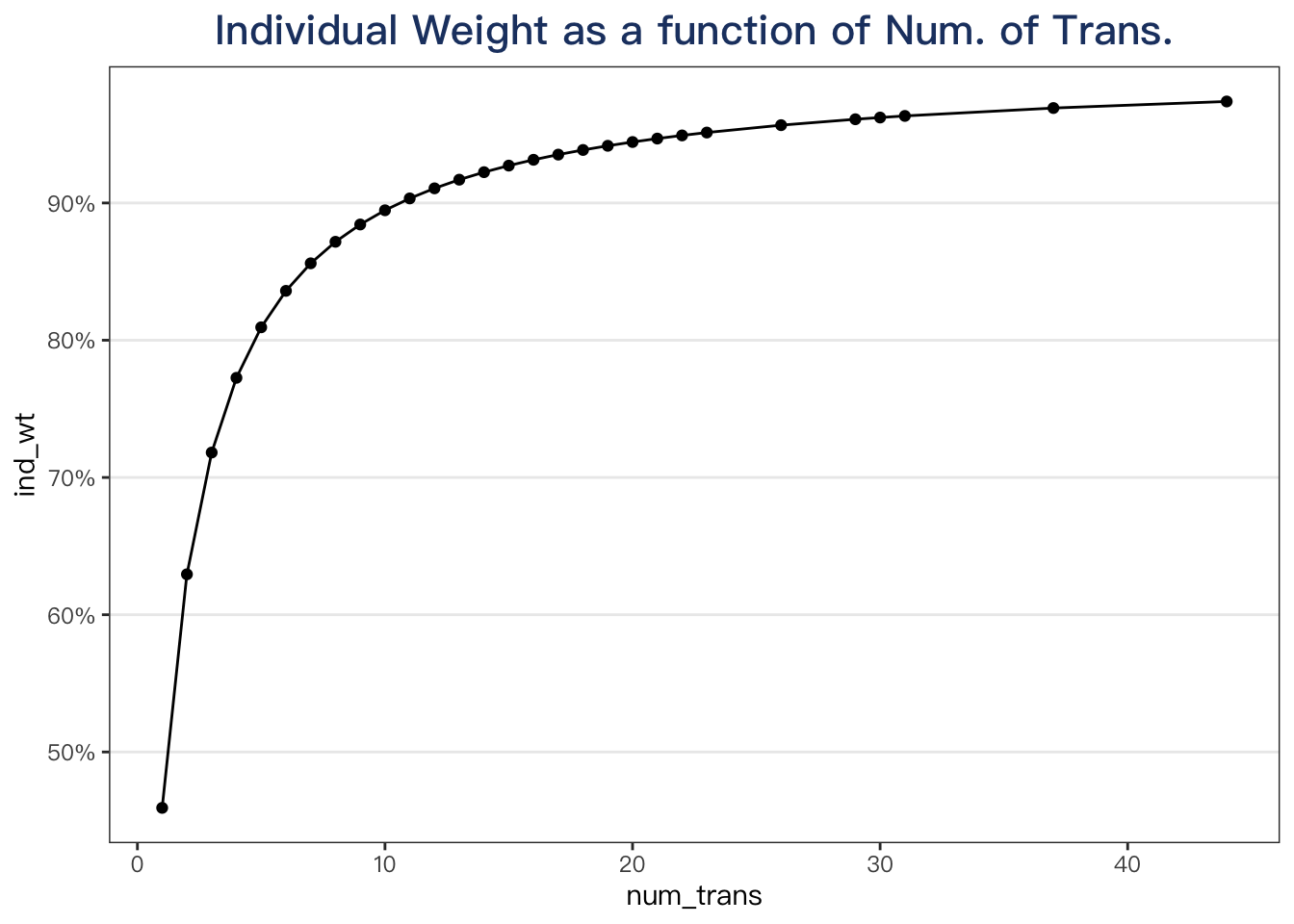
Understand weighted average
Calculate the weight for the given individual’s observed average,
# calculate the weight for the given individual's observed average
cal_ind_wt <- function(param_vec, num_trans) {
  p = param_vec[1]
  q = param_vec[2]
  r = param_vec[3]
  x = num_trans

  unname(
    (p*x) / (p*x + q - 1)
  )
}
Calculate the population mean,
cal_pop_mean <- function(param_vec) {
  p <- param_vec[1]
  q <- param_vec[2]
  r <- param_vec[3]

  if (q < 1) {
    stop("q must be greater than 1!")
  }

  # return
  res <- (p * r) / (q - 1)

  unname(res)
}

# what is the pop mean
pop_mean_spend <- cal_pop_mean(params)

pop_mean_spend
## [1] 3050.065
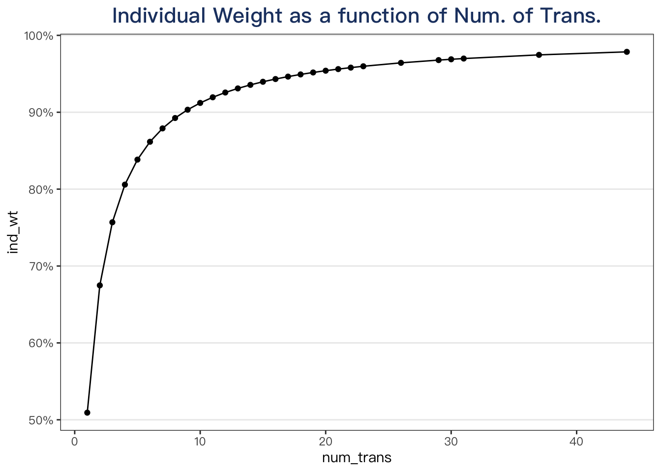
Now let’s compute the weight for each customer,
plotdata <- spend_cbs_data %>%
  select(cust, is_single, num_trans, avg_spend) %>%
  mutate(ind_wt = cal_ind_wt(params, num_trans)) %>%
  mutate(pop_wt = 1 - ind_wt)

set.seed(123)

plotdata %>%
  slice_sample(n = 10) %>%
  mutate(across(ends_with("wt"), fmt_pct)) %>%
  mutate(avg_spend = fmt_comma(avg_spend)) %>%
  print_kbl(cap = "weight for individual vs. weight for pop")
| cust | is_single | num_trans | avg_spend | ind_wt | pop_wt |
|---|---|---|---|---|---|
| uid4895 | FALSE | 3 | 1,574 | 76% | 24% |
| uid1199 | TRUE | 1 | 6,809 | 51% | 49% |
| uid0433 | FALSE | 4 | 1,971 | 81% | 19% |
| uid4051 | FALSE | 12 | 2,022 | 93% | 7% |
| uid2552 | TRUE | 1 | 3,132 | 51% | 49% |
| uid2792 | TRUE | 1 | 280 | 51% | 49% |
| uid2829 | TRUE | 1 | 4,485 | 51% | 49% |
| uid2348 | TRUE | 1 | 1,730 | 51% | 49% |
| uid1525 | FALSE | 4 | 2,005 | 81% | 19% |
| uid3588 | TRUE | 1 | 1,706 | 51% | 49% |
plotdata %>%
  distinct(num_trans, .keep_all = TRUE) %>%
  select(num_trans, ind_wt) %>%
  ggplot(aes(x = num_trans, y = ind_wt)) +
  geom_point() +
  geom_line() +
  scale_y_continuous(labels = fmt_pct) +
  labs(title = "Individual Weight as a function of Num. of Trans.")
Parameter Estimation (without the 1st trans.)
params2 <- CLVTools::gg(clv.data = dclv, remove.first.transaction = TRUE) %>% coef

params2
##           p           q       gamma
##    1.309883    2.542147 3975.335041
plotdata <- spend_cbs_data %>%
  select(cust, is_single, num_trans, avg_spend) %>%
  mutate(ind_wt = cal_ind_wt(params2, num_trans)) %>%
  mutate(pop_wt = 1 - ind_wt)

plotdata %>%
  distinct(num_trans, .keep_all = TRUE) %>%
  select(num_trans, ind_wt) %>%
  ggplot(aes(x = num_trans, y = ind_wt)) +
  geom_point() +
  geom_line() +
  scale_y_continuous(labels = fmt_pct) +
  labs(title = "Individual Weight as a function of Num. of Trans.")